PyData Paris 2025
Skrub - Machine learning with dataframes
Riccardo Cappuzzo, Jérôme Dockès, Guillaume Lemaître
Inria P16, probabl.
2025-10-01
whoami
I am a research engineer at Inria as part of the P16 project, and I am the lead developer of skrub
![]()
I’m Italian, but I don’t drink coffee, wine, and I like pizza with fries
![]()
I did my PhD in Côte d’Azur, and I moved away because it was too sunny and I don’t like the sea
![]()


Boost your productivity with skrub!
Skrub simplifies many tedious data preparation operations
skrub compatibility
- Skrub is fully compatible with pandas and polars
- Skrub transformers are fully compatible with scikit-learn
An example pipeline
- Gather some data
- Explore the data
- Preprocess the data
- Perform feature engineering
- Build a scikit-learn pipeline
- ???
- Profit?

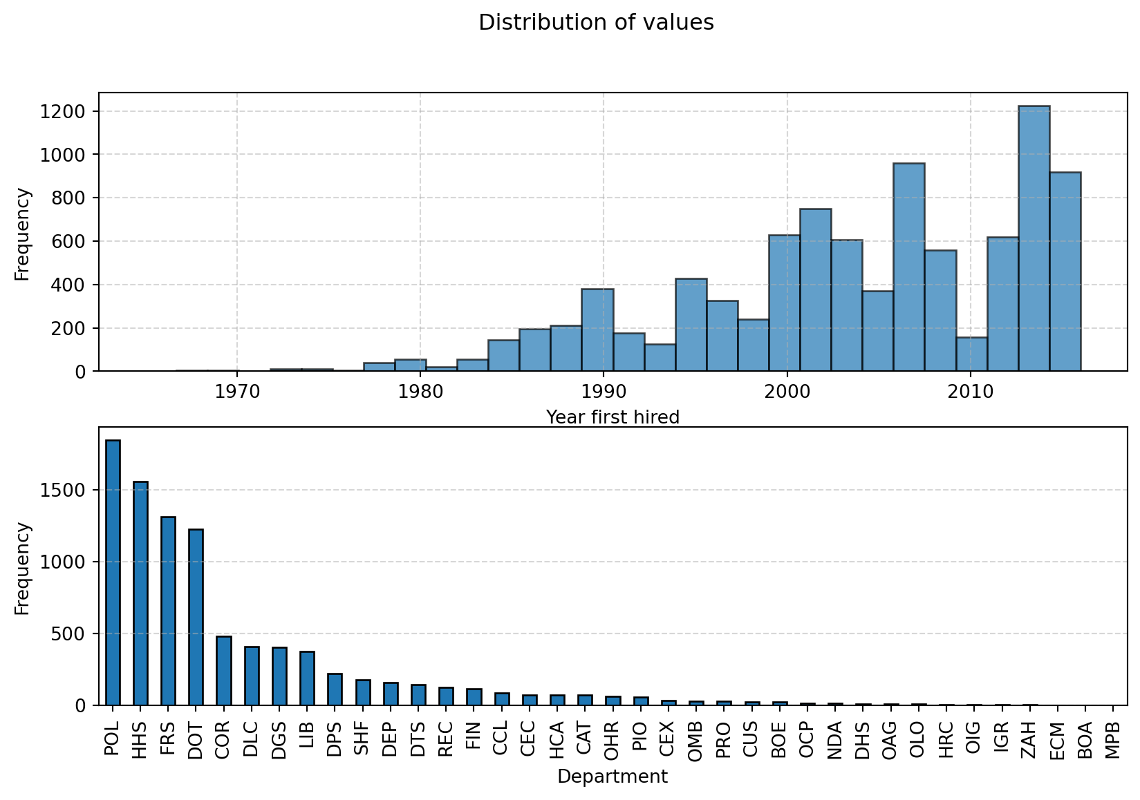
Exploring the data
import pandas as pd
import matplotlib.pyplot as plt
import skrub

dataset = skrub.datasets.fetch_employee_salaries()
employees, salaries = dataset.X, dataset.y

df = pd.DataFrame(employees)

# Plot the distribution of the numerical values using a histogram
fig, axs = plt.subplots(2,1, figsize=(10, 6))
ax1, ax2 = axs

ax1.hist(df['year_first_hired'], bins=30, edgecolor='black', alpha=0.7)
ax1.set_xlabel('Year first hired')
ax1.set_ylabel('Frequency')
ax1.grid(True, linestyle='--', alpha=0.5)

# Count the frequency of each category
category_counts = df['department'].value_counts()

# Create a bar plot
category_counts.plot(kind='bar', edgecolor='black', ax=ax2)

# Add labels and title
ax2.set_xlabel('Department')
ax2.set_ylabel('Frequency')
ax2.grid(True, linestyle='--', axis='y', alpha=0.5)  # Add grid lines for y-axis

fig.suptitle("Distribution of values")

# Show the plot
plt.show()
Exploring the data
Exploring the data with skrub
Main features:
- Obtain high-level statistics about the data
- Explore the distribution of values and find outliers
- Discover highly correlated columns
- Export and share the report as an
htmlfile
Data cleaning with pandas/polars: setup
import pandas as pd
import numpy as np

data = {
    "Int": [2, 3, 2],  # Multiple unique values
    "Const str": ["x", "x", "x"],  # Single unique value
    "Str": ["foo", "bar", "baz"],  # Multiple unique values
    "All nan": [np.nan, np.nan, np.nan],  # All missing values
    "All empty": ["", "", ""],  # All empty strings
    "Date": ["01 Jan 2023", "02 Jan 2023", "03 Jan 2023"],
}

df_pd = pd.DataFrame(data)
display(df_pd)| Int | Const str | Str | All nan | All empty | Date | |
|---|---|---|---|---|---|---|
| 0 | 2 | x | foo | NaN | 01 Jan 2023 | |
| 1 | 3 | x | bar | NaN | 02 Jan 2023 | |
| 2 | 2 | x | baz | NaN | 03 Jan 2023 |
import polars as pl
import numpy as np
data = {
    "Int": [2, 3, 2],  # Multiple unique values
    "Const str": ["x", "x", "x"],  # Single unique value
    "Str": ["foo", "bar", "baz"],  # Multiple unique values
    "All nan": [np.nan, np.nan, np.nan],  # All missing values
    "All empty": ["", "", ""],  # All empty strings
    "Date": ["01 Jan 2023", "02 Jan 2023", "03 Jan 2023"],
}

df_pl = pl.DataFrame(data)
display(df_pl)
shape: (3, 6)
| Int | Const str | Str | All nan | All empty | Date |
|---|---|---|---|---|---|
| i64 | str | str | f64 | str | str |
| 2 | "x" | "foo" | NaN | "" | "01 Jan 2023" |
| 3 | "x" | "bar" | NaN | "" | "02 Jan 2023" |
| 2 | "x" | "baz" | NaN | "" | "03 Jan 2023" |
Nulls, datetimes, constant columns with pandas/polars
# Parse the datetime strings with a specific format
df_pd['Date'] = pd.to_datetime(df_pd['Date'], format='%d %b %Y')

# Drop columns with only a single unique value
df_pd_cleaned = df_pd.loc[:, df_pd.nunique(dropna=True) > 1]

# Function to drop columns with only missing values or empty strings
def drop_empty_columns(df):
    # Drop columns with only missing values
    df_cleaned = df.dropna(axis=1, how='all')
    # Drop columns with only empty strings
    empty_string_cols = df_cleaned.columns[df_cleaned.eq('').all()]
    df_cleaned = df_cleaned.drop(columns=empty_string_cols)
    return df_cleaned

# Apply the function to the DataFrame
df_pd_cleaned = drop_empty_columns(df_pd_cleaned)
# Parse the datetime strings with a specific format
df_pl = df_pl.with_columns([
pl.col("Date").str.strptime(pl.Date, "%d %b %Y", strict=False).alias("Date")
])
# Drop columns with only a single unique value
df_pl_cleaned = df_pl.select([
col for col in df_pl.columns if df_pl[col].n_unique() > 1
])
# Import selectors for dtype selection
import polars.selectors as cs
# Drop columns with only missing values or only empty strings
def drop_empty_columns(df):
all_nan = df.select(
[
col for col in df.select(cs.numeric()).columns if
df [col].is_nan().all()
]
).columns
all_empty = df.select(
[
col for col in df.select(cs.string()).columns if
(df[col].str.strip_chars().str.len_chars()==0).all()
]
).columns
to_drop = all_nan + all_empty
return df.drop(to_drop)
df_pl_cleaned = drop_empty_columns(df_pl_cleaned)Data cleaning with skrub.Cleaner
Encoding datetime features with pandas/polars
import pandas as pd
data = {
    'date': ['2023-01-01 12:34:56', '2023-02-15 08:45:23', '2023-03-20 18:12:45'],
    'value': [10, 20, 30]
}
df_pd = pd.DataFrame(data)
datetime_column = "date"
df_pd[datetime_column] = pd.to_datetime(df_pd[datetime_column], errors='coerce')

df_pd['year'] = df_pd[datetime_column].dt.year
df_pd['month'] = df_pd[datetime_column].dt.month
df_pd['day'] = df_pd[datetime_column].dt.day
df_pd['hour'] = df_pd[datetime_column].dt.hour
df_pd['minute'] = df_pd[datetime_column].dt.minute
df_pd['second'] = df_pd[datetime_column].dt.second
import polars as pl
data = {
'date': ['2023-01-01 12:34:56', '2023-02-15 08:45:23', '2023-03-20 18:12:45'],
'value': [10, 20, 30]
}
df_pl = pl.DataFrame(data)
df_pl = df_pl.with_columns(date=pl.col("date").str.to_datetime())
df_pl = df_pl.with_columns(
year=pl.col("date").dt.year(),
month=pl.col("date").dt.month(),
day=pl.col("date").dt.day(),
hour=pl.col("date").dt.hour(),
minute=pl.col("date").dt.minute(),
second=pl.col("date").dt.second(),
)Encoding datetime features with skrub.DatetimeEncoder
shape: (3, 7)
┌───────────┬────────────┬──────────┬───────────┬─────────────┬─────────────┬────────────────────┐
│ date_year ┆ date_month ┆ date_day ┆ date_hour ┆ date_minute ┆ date_second ┆ date_total_seconds │
│ ---       ┆ ---        ┆ ---      ┆ ---       ┆ ---         ┆ ---         ┆ ---                │
│ f32       ┆ f32        ┆ f32      ┆ f32       ┆ f32         ┆ f32         ┆ f32                │
╞═══════════╪════════════╪══════════╪═══════════╪═════════════╪═════════════╪════════════════════╡
│ 2023.0    ┆ 1.0        ┆ 1.0      ┆ 12.0      ┆ 34.0        ┆ 56.0        ┆ 1.6726e9           │
│ 2023.0    ┆ 2.0        ┆ 15.0     ┆ 8.0       ┆ 45.0        ┆ 23.0        ┆ 1.6765e9           │
│ 2023.0    ┆ 3.0        ┆ 20.0     ┆ 18.0      ┆ 12.0        ┆ 45.0        ┆ 1.6793e9           │
└───────────┴────────────┴──────────┴───────────┴─────────────┴─────────────┴────────────────────┘
What periodic features look like
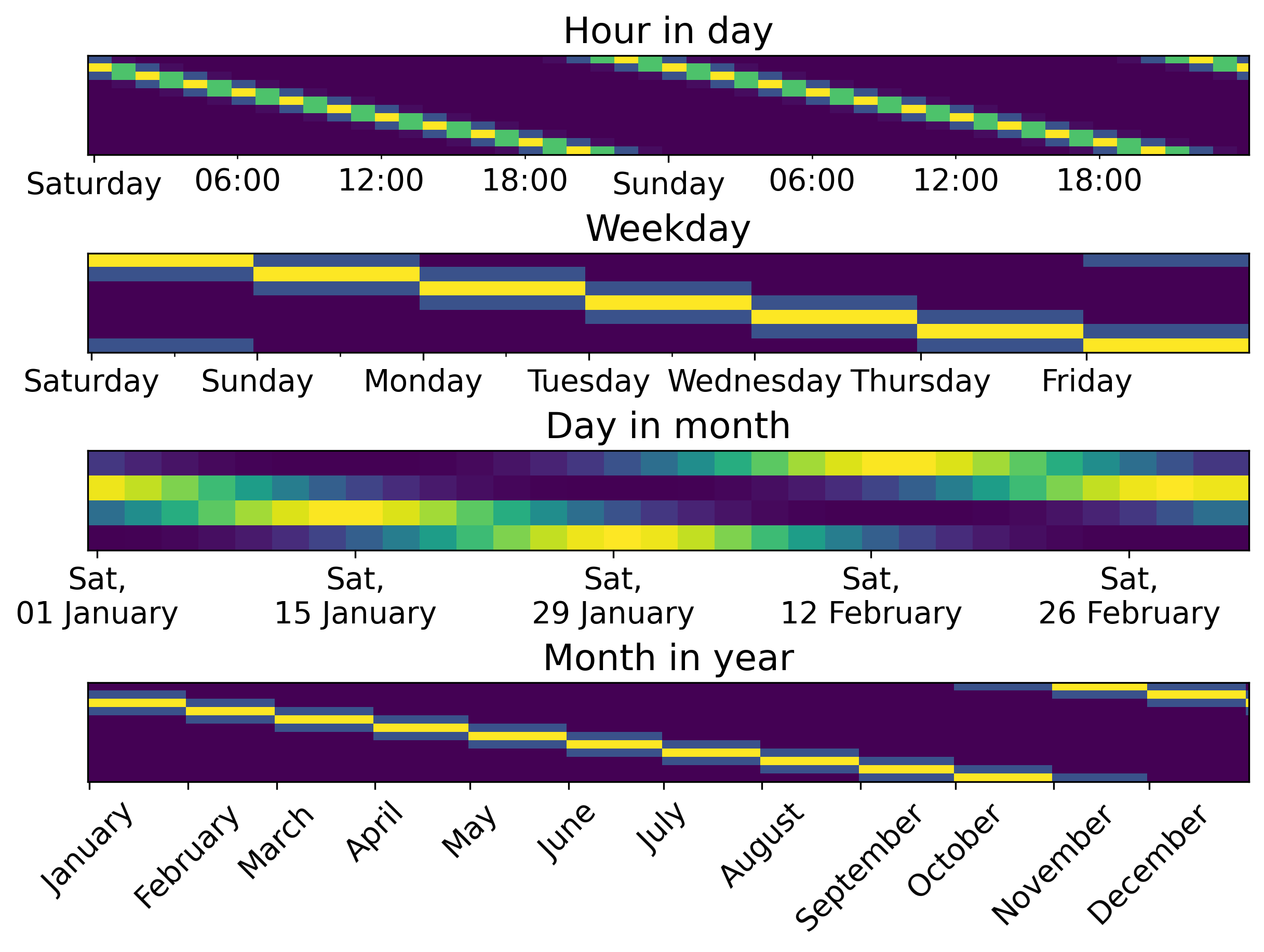
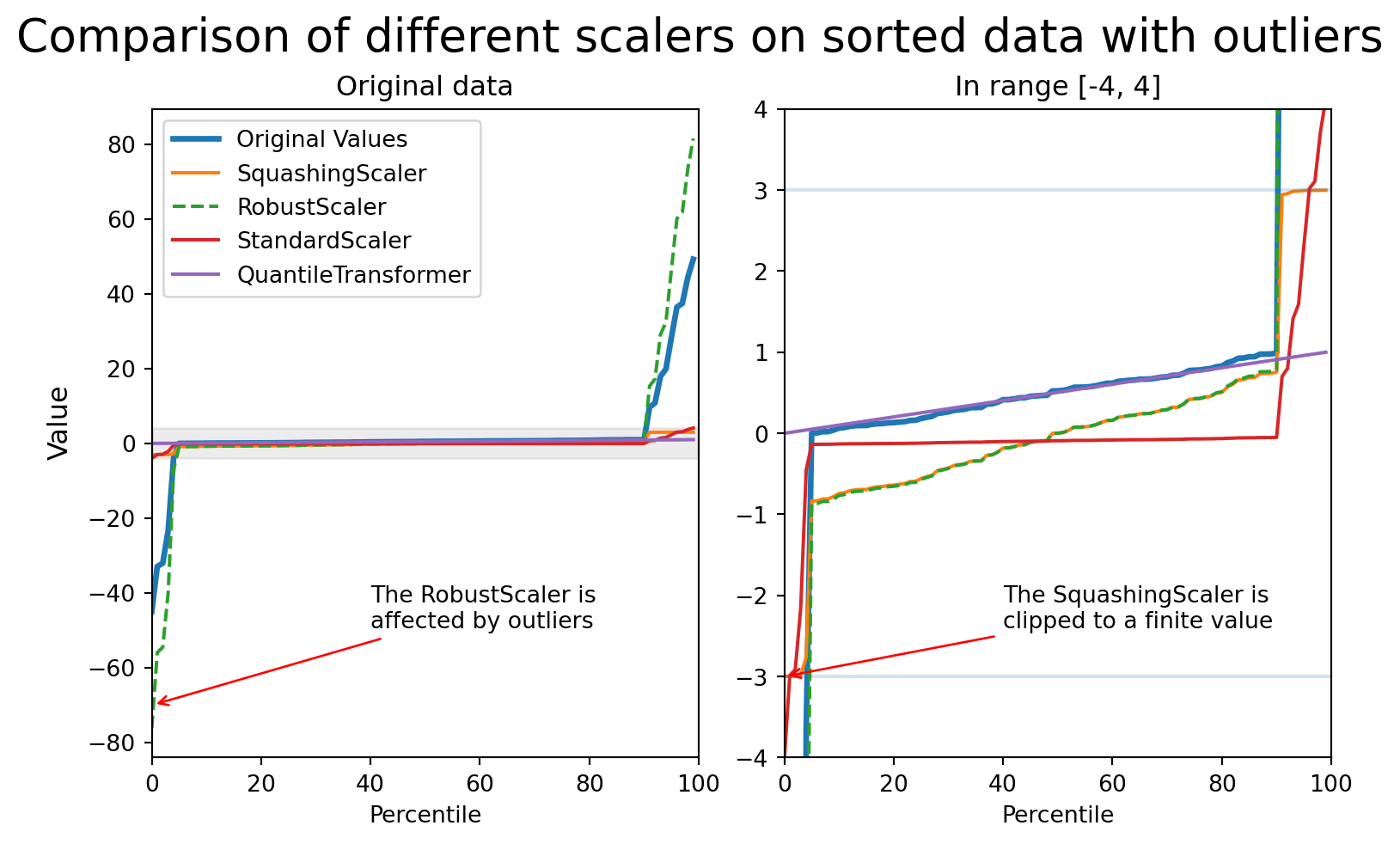
Encoding numerical features with skrub.SquashingScaler
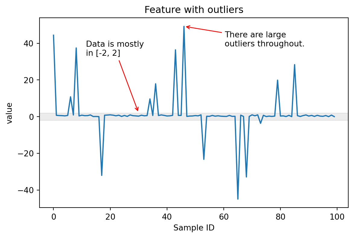
Encoding numerical features with skrub.SquashingScaler
Encoding categorical (string/text) features
Categorical features have a “cardinality”: the number of unique values
- Low cardinality:
OneHotEncoder - High cardinality (>40 unique values):
skrub.StringEncoder - Text:
skrub.TextEncoderand pretrained models from HuggingFace Hub
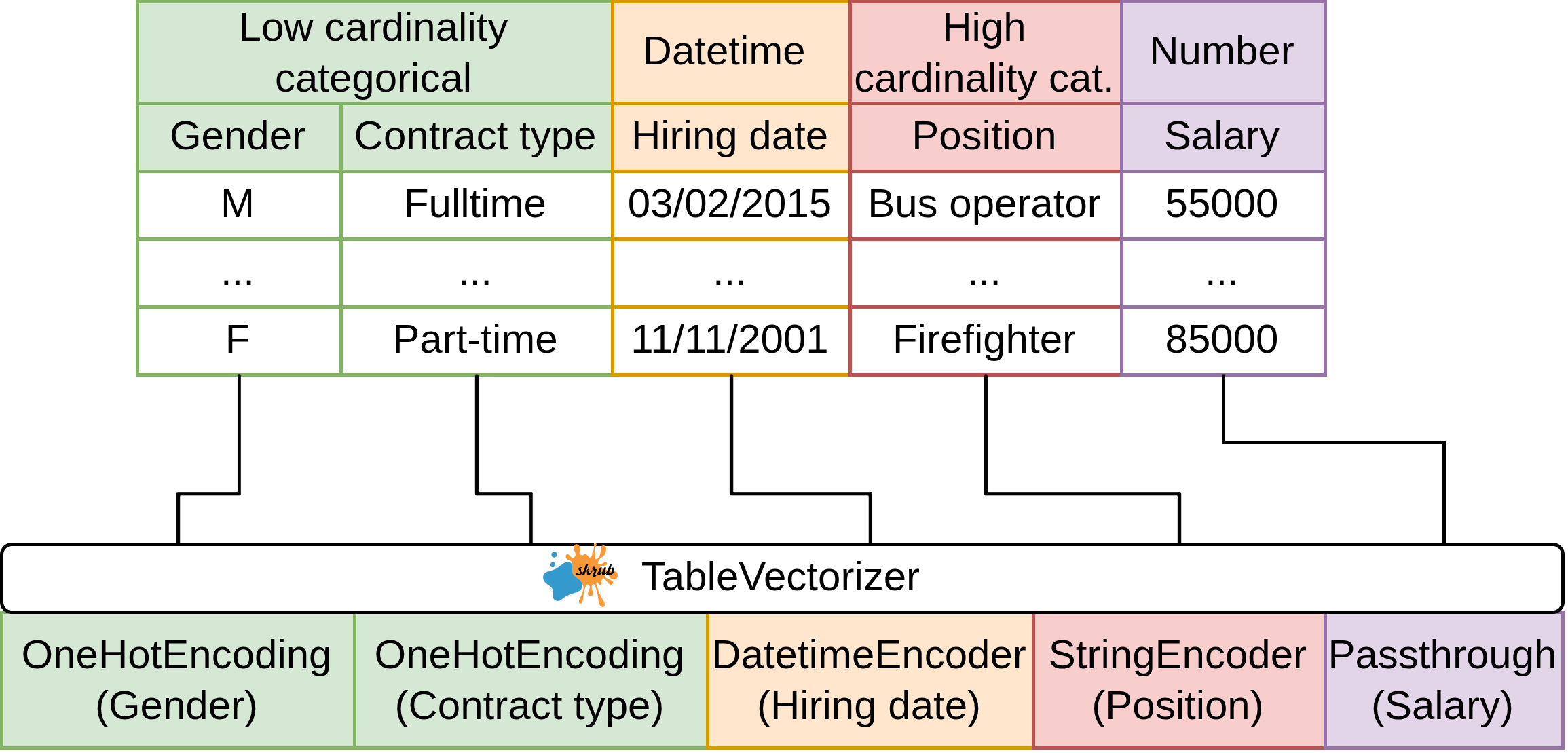
Encoding all the features: TableVectorizer
- Apply the
Cleanerto all columns - Split columns by dtype and # of unique values
- Encode each column separately
Encoding all the features: TableVectorizer
Build a predictive pipeline
Build a predictive pipeline
from sklearn.linear_model import Ridge
from sklearn.pipeline import make_pipeline
from sklearn.preprocessing import StandardScaler, OneHotEncoder
from sklearn.impute import SimpleImputer
from sklearn.compose import make_column_selector as selector
from sklearn.compose import make_column_transformer

categorical_columns = selector(dtype_include=object)(employees)
numerical_columns = selector(dtype_exclude=object)(employees)

ct = make_column_transformer(
      (StandardScaler(),
       numerical_columns),
      (OneHotEncoder(handle_unknown="ignore"),
       categorical_columns))

model = make_pipeline(ct, SimpleImputer(), Ridge())
Build a predictive pipeline with tabular_pipeline
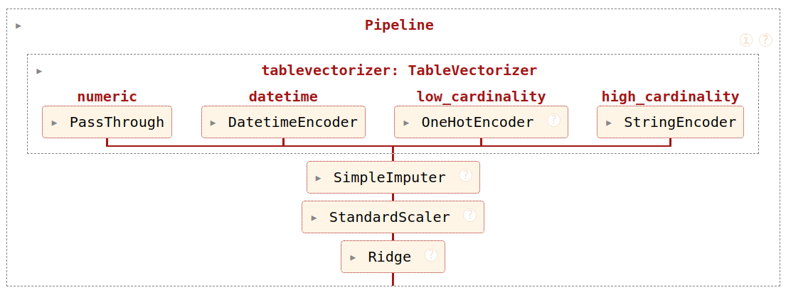

We now have a pipeline!
- Gather some data
- Explore the data
TableReport
- Pre-process the data
Cleaner,ToDatetime…
- Perform feature engineering
TableVectorizer,SquashingScaler,TextEncoder,StringEncoder…
- Build a scikit-learn pipeline
tabular_pipeline…
- ???
- Profit 📈
What if this is not enough??
What if…
- Your data is spread over multiple tables?
- You want to avoid data leakage?
- You want to tune more than just the hyperparameters of your model?
- You want to guarantee that your pipeline is replayed exactly on new data?
When a normal pipe is not enough…
… the skrub DataOps come to the rescue 🚒
DataOps…
- Extend the
scikit-learnmachinery to complex multi-table operations, and take care of data leakage - Track all operations with a computational graph (a Data Ops plan)
- Are transparent and give direct access to the underlying object
- Allow tuning any operation in the Data Ops plan
- Guarantee that all operations are reproducible
- Can be persisted and shared easily
How do DataOps work, though?
DataOps wrap around user operations, where user operations are:
- any dataframe operation (e.g., merge, group by, aggregate etc.)
- scikit-learn estimators (a Random Forest, RidgeCV etc.)
- custom user code (load data from a path, fetch from an URL etc.)
Important
DataOps record user operations, so that they can later be replayed in the same order and with the same arguments on unseen data.
Starting with the DataOps
basketsandproductsrepresent inputs to the pipeline.- Skrub tracks
Xandyso that training and test splits are never mixed.
Applying a transformer
Executing dataframe operations
Applying a ML model
Inspecting the Data Ops plan
Each node:
- Shows a preview of the data resulting from the operation
- Reports the location in the code where the code is defined
- Shows the run time of the node
The plan is exported as HTML + JS (no need for kernels).
Exporting the plan in a learner
The Learner is a stand-alone object that works like a scikit-learn estimator that takes a dictionary as input rather than just X and y.
Then, the learner can be pickled …
… loaded and applied to new data:
array([0, 0, 0, ..., 0, 0, 0], shape=(31549,))Hyperparameter tuning in a Data Plan
Skrub implements four choose_* functions:
choose_from: select from the given list of optionschoose_int: select an integer within a rangechoose_float: select a float within a rangechoose_bool: select a booloptional: chooses whether to execute the given operation
Tuning in scikit-learn can be complex
pipe = Pipeline([("dim_reduction", PCA()), ("regressor", Ridge())])
grid = [
    {
        "dim_reduction": [PCA()],
        "dim_reduction__n_components": [10, 20, 30],
        "regressor": [Ridge()],
        "regressor__alpha": loguniform(0.1, 10.0),
    },
    {
        "dim_reduction": [SelectKBest()],
        "dim_reduction__k": [10, 20, 30],
        "regressor": [Ridge()],
        "regressor__alpha": loguniform(0.1, 10.0),
    },
    {
        "dim_reduction": [PCA()],
        "dim_reduction__n_components": [10, 20, 30],
        "regressor": [RandomForestRegressor()],
        "regressor__n_estimators": loguniform(20, 200),
    },
    {
        "dim_reduction": [SelectKBest()],
        "dim_reduction__k": [10, 20, 30],
        "regressor": [RandomForestRegressor()],
        "regressor__n_estimators": loguniform(20, 200),
    },
]
Tuning with DataOps is simple!
dim_reduction = X.skb.apply(
    skrub.choose_from(
        {
            "PCA": PCA(n_components=skrub.choose_int(10, 30)),
            "SelectKBest": SelectKBest(k=skrub.choose_int(10, 30))
        }, name="dim_reduction"
    )
)
regressor = dim_reduction.skb.apply(
    skrub.choose_from(
        {
            "Ridge": Ridge(alpha=skrub.choose_float(0.1, 10.0, log=True)),
            "RandomForest": RandomForestRegressor(
                n_estimators=skrub.choose_int(20, 200, log=True)
            )
        }, name="regressor"
    )
)
Run hyperparameter search
Tuning with DataOps is not limited to estimators
'- choose_from([<Expr [\'col("grade").mean()\'] at 0x15B34D510>, <Expr [\'col("grade").count()\'] at 0x15B34FE20>]): [<Expr [\'col("grade").mean()\'] at 0x15B34D510>, <Expr [\'col("grade").count()\'] at 0x15B34FE20>]\n'A parallel coordinate plot to explore hyperparameters
More information about the Data Ops
- Skrub example gallery
- Skrub user guide
- Tutorial on timeseries forecasting at Euroscipy 2025
- Kaggle notebook on the Titanic survival challenge
Wrapping up


Getting involved
Do you want to learn more?
Follow skrub on:
Star skrub on GitHub, or contribute directly:
Sprint on Thursday!!!
We’re hiring!!
Come talk to me or go to the P16 booth
tl;dw: skrub
- interactive data exploration:
TableReport - automated pre-processing of pandas and polars dataframes:
Cleaner - powerful feature engineering:
TableVectorizer,tabular_pipeline - column- and dataframe-level operations:
ApplyToCols, selectors - DataOps, plans, hyperparameter tuning, (almost) no leakage
Fine-grained column transformations with ApplyToCols
import pandas as pd
from sklearn.compose import make_column_selector as selector
from sklearn.compose import make_column_transformer
from sklearn.preprocessing import StandardScaler, OneHotEncoder

df = pd.DataFrame({"text": ["foo", "bar", "baz"], "number": [1, 2, 3]})

categorical_columns = selector(dtype_include=object)(df)
numerical_columns = selector(dtype_exclude=object)(df)

ct = make_column_transformer(
      (StandardScaler(),
       numerical_columns),
      (OneHotEncoder(handle_unknown="ignore"),
       categorical_columns))
transformed = ct.fit_transform(df)
transformed
array([[-1.22474487, 0. , 0. , 1. ],
[ 0. , 1. , 0. , 0. ],
[ 1.22474487, 0. , 1. , 0. ]])Fine-grained column transformations with ApplyToCols
import skrub.selectors as s
from sklearn.pipeline import make_pipeline
from skrub import ApplyToCols

numeric = ApplyToCols(StandardScaler(), cols=s.numeric())
string = ApplyToCols(OneHotEncoder(sparse_output=False), cols=s.string())

transformed = make_pipeline(numeric, string).fit_transform(df)
transformed| text_bar | text_baz | text_foo | number | |
|---|---|---|---|---|
| 0 | 0.0 | 0.0 | 1.0 | -1.224745 |
| 1 | 1.0 | 0.0 | 0.0 | 0.000000 |
| 2 | 0.0 | 1.0 | 0.0 | 1.224745 |

https://skrub-data.org/skrub-materials/