EDF Talk: Skrub

Machine learning with dataframes

Riccardo Cappuzzo

Inria P16

2025-09-16

Boost your productivity with skrub!

Skrub simplifies many tedious data preparation operations

A teaser for later…

Inspect all the steps of your pipeline: Execution report

A teaser for later…

Explore your hyperparameter search space

skrub compatibility

skrub is fully compatible with pandas and polars
skrub transformers are fully compatible with scikit-learn

An example pipeline

Gather some data
Explore the data
Preprocess the data
Perform feature engineering
Build a scikit-learn pipeline
???
Profit?

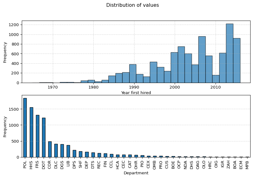
Exploring the data

import pandas as pd
import matplotlib.pyplot as plt
import skrub

dataset = skrub.datasets.fetch_employee_salaries()
employees, salaries = dataset.X, dataset.y

df = pd.DataFrame(employees)

# Plot the distribution of the numerical values using a histogram
fig, axs = plt.subplots(2,1, figsize=(10, 6))
ax1, ax2 = axs

ax1.hist(df['year_first_hired'], bins=30, edgecolor='black', alpha=0.7)
ax1.set_xlabel('Year first hired')
ax1.set_ylabel('Frequency')
ax1.grid(True, linestyle='--', alpha=0.5)

# Count the frequency of each category
category_counts = df['department'].value_counts()

# Create a bar plot
category_counts.plot(kind='bar', edgecolor='black', ax=ax2)

# Add labels and title
ax2.set_xlabel('Department')
ax2.set_ylabel('Frequency')
ax2.grid(True, linestyle='--', axis='y', alpha=0.5)  # Add grid lines for y-axis

fig.suptitle("Distribution of values")

# Show the plot
plt.show()

Exploring the data

Exploring the data with `skrub`

from skrub import TableReport
TableReport(employee_salaries)

Preview

Main features:

Obtain high-level statistics about the data
Explore the distribution of values and find outliers
Discover highly correlated columns
Export and share the report as an html file

More examples

import pandas as pd
import numpy as np
data = {
    'Constant int': [1, 1, 1],  # Single unique value
    'B': [2, 3, 2],  # Multiple unique values
    'Constant str': ['x', 'x', 'x'],  # Single unique value
    'D': [4, 5, 6],  # Multiple unique values
    'All nan': [np.nan, np.nan, np.nan],  # All missing values 
    'All empty': ['', '', ''],  # All empty strings
    'Date': ['01/01/2023', '02/01/2023', '03/01/2023'],
}

df_pd = pd.DataFrame(data)
display(df_pd)

	Constant int	B	Constant str	D	All nan	Date
0	1	2	x	4	NaN	01/01/2023
1	1	3	x	5	NaN	02/01/2023
2	1	2	x	6	NaN	03/01/2023

import polars as pl
import numpy as np
data = {
    'Constant int': [1, 1, 1],  # Single unique value
    'B': [2, 3, 2],  # Multiple unique values
    'Constant str': ['x', 'x', 'x'],  # Single unique value
    'D': [4, 5, 6],  # Multiple unique values
    'All nan': [np.nan, np.nan, np.nan],  # All missing values 
    'All empty': ['', '', ''],  # All empty strings
    'Date': ['01/01/2023', '02/01/2023', '03/01/2023'],
}

df_pl = pl.DataFrame(data)
display(df_pl)

shape: (3, 7)

Constant int	B	Constant str	D	All nan	All empty	Date
i64	i64	str	i64	f64	str	str
1	2	"x"	4	NaN	""	"01/01/2023"
1	3	"x"	5	NaN	""	"02/01/2023"
1	2	"x"	6	NaN	""	"03/01/2023"

Nulls, datetimes, constant columns with pandas/polars

Pandas
Polars

# Parse the datetime strings with a specific format
df_pd['Date'] = pd.to_datetime(df_pd['Date'], format='%d/%m/%Y')

# Drop columns with only a single unique value
df_pd_cleaned = df_pd.loc[:, df_pd.nunique(dropna=True) > 1]

# Function to drop columns with only missing values or empty strings
def drop_empty_columns(df):
    # Drop columns with only missing values
    df_cleaned = df.dropna(axis=1, how='all')
    # Drop columns with only empty strings
    empty_string_cols = df_cleaned.columns[df_cleaned.eq('').all()]
    df_cleaned = df_cleaned.drop(columns=empty_string_cols)
    return df_cleaned

# Apply the function to the DataFrame
df_pd_cleaned = drop_empty_columns(df_pd_cleaned)

# Parse the datetime strings with a specific format
df_pl = df_pl.with_columns([
    pl.col("Date").str.strptime(pl.Date, "%d/%m/%Y", strict=False).alias("Date")
])

# Drop columns with only a single unique value
df_pl_cleaned = df_pl.select([
    col for col in df_pl.columns if df_pl[col].n_unique() > 1
])

# Import selectors for dtype selection
import polars.selectors as cs

# Drop columns with only missing values or only empty strings
def drop_empty_columns(df):
    all_nan = df.select(
        [
            col for col in df.select(cs.numeric()).columns if 
            df [col].is_nan().all()
        ]
    ).columns
    
    all_empty = df.select(
        [
            col for col in df.select(cs.string()).columns if 
            (df[col].str.strip_chars().str.len_chars()==0).all()
        ]
    ).columns

    to_drop = all_nan + all_empty

    return df.drop(to_drop)

df_pl_cleaned = drop_empty_columns(df_pl_cleaned)

Data cleaning with `skrub.Cleaner`

Pandas
Polars

from skrub import Cleaner
cleaner = Cleaner(drop_if_constant=True, datetime_format='%d/%m/%Y')
df_cleaned = cleaner.fit_transform(df_pd)
display(df_cleaned)

	B	D	Date
0	2	4	2023-01-01
1	3	5	2023-01-02
2	2	6	2023-01-03

from skrub import Cleaner
cleaner = Cleaner(drop_if_constant=True, datetime_format='%d/%m/%Y')
df_cleaned = cleaner.fit_transform(df_pl)
display(df_cleaned)

shape: (3, 3)

B	D	Date
i64	i64	date
2	4	2023-01-01
3	5	2023-01-02
2	6	2023-01-03

Comparison

Pandas
Polars

print(df_pd_cleaned)

   B  D       Date
0  2  4 2023-01-01
1  3  5 2023-01-02
2  2  6 2023-01-03

print(df_cleaned)

   B  D       Date
0  2  4 2023-01-01
1  3  5 2023-01-02
2  2  6 2023-01-03

print(df_pl_cleaned)

shape: (3, 3)
┌─────┬─────┬────────────┐
│ B   ┆ D   ┆ Date       │
│ --- ┆ --- ┆ ---        │
│ i64 ┆ i64 ┆ date       │
╞═════╪═════╪════════════╡
│ 2   ┆ 4   ┆ 2023-01-01 │
│ 3   ┆ 5   ┆ 2023-01-02 │
│ 2   ┆ 6   ┆ 2023-01-03 │
└─────┴─────┴────────────┘

print(df_cleaned)

shape: (3, 3)
┌─────┬─────┬────────────┐
│ B   ┆ D   ┆ Date       │
│ --- ┆ --- ┆ ---        │
│ i64 ┆ i64 ┆ date       │
╞═════╪═════╪════════════╡
│ 2   ┆ 4   ┆ 2023-01-01 │
│ 3   ┆ 5   ┆ 2023-01-02 │
│ 2   ┆ 6   ┆ 2023-01-03 │
└─────┴─────┴────────────┘

Encoding datetime features with pandas/polars

Pandas
Polars

import pandas as pd
data = {
    'date': ['2023-01-01 12:34:56', '2023-02-15 08:45:23', '2023-03-20 18:12:45'],
    'value': [10, 20, 30]
}
df_pd = pd.DataFrame(data)
datetime_column = "date"
df_pd[datetime_column] = pd.to_datetime(df_pd[datetime_column], errors='coerce')

df_pd['year'] = df_pd[datetime_column].dt.year
df_pd['month'] = df_pd[datetime_column].dt.month
df_pd['day'] = df_pd[datetime_column].dt.day
df_pd['hour'] = df_pd[datetime_column].dt.hour
df_pd['minute'] = df_pd[datetime_column].dt.minute
df_pd['second'] = df_pd[datetime_column].dt.second

import polars as pl
data = {
    'date': ['2023-01-01 12:34:56', '2023-02-15 08:45:23', '2023-03-20 18:12:45'],
    'value': [10, 20, 30]
}
df_pl = pl.DataFrame(data)
df_pl = df_pl.with_columns(date=pl.col("date").str.to_datetime())

df_pl = df_pl.with_columns(
    year=pl.col("date").dt.year(),
    month=pl.col("date").dt.month(),
    day=pl.col("date").dt.day(),
    hour=pl.col("date").dt.hour(),
    minute=pl.col("date").dt.minute(),
    second=pl.col("date").dt.second(),
)

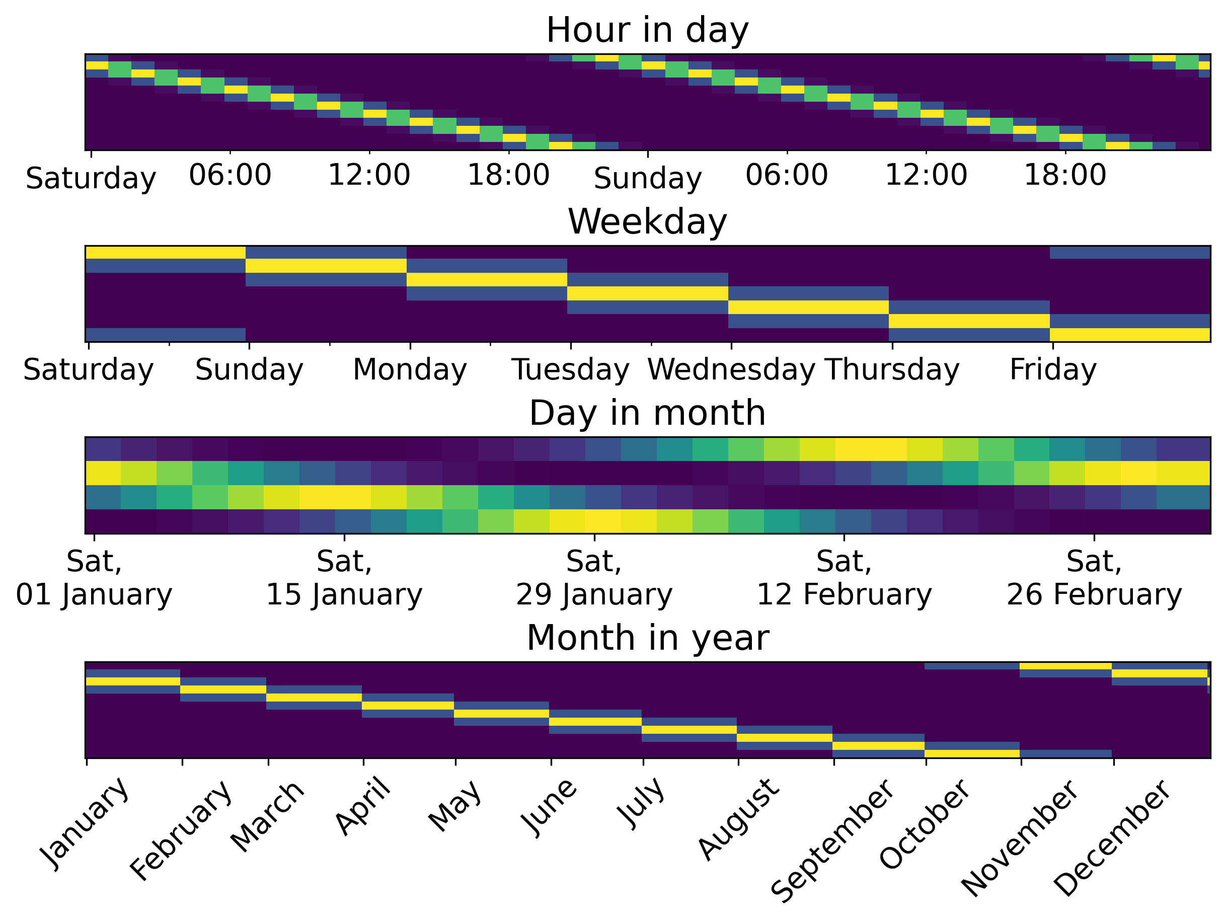
Adding periodic features with pandas/polars

Pandas
Polars

df_pd['hour_sin'] = np.sin(2 * np.pi * df_pd['hour'] / 24)
df_pd['hour_cos'] = np.cos(2 * np.pi * df_pd['hour'] / 24)

df_pd['month_sin'] = np.sin(2 * np.pi * df_pd['month'] / 12)
df_pd['month_cos'] = np.cos(2 * np.pi * df_pd['month'] / 12)

df_pl = df_pl.with_columns(
    hour_sin = np.sin(2 * np.pi * pl.col("hour") / 24),
    hour_cos = np.cos(2 * np.pi * pl.col("hour") / 24),
    
    month_sin = np.sin(2 * np.pi * pl.col("month") / 12),
    month_cos = np.cos(2 * np.pi * pl.col("month") / 12),
)

Encoding datetime features `skrub.DatetimeEncoder`

from skrub import DatetimeEncoder, ToDatetime

X_date = ToDatetime().fit_transform(df["date"])
de = DatetimeEncoder(periodic_encoding="circular")
X_enc = de.fit_transform(X_date)
print(X_enc)

shape: (3, 8)
┌───────────┬────────────┬────────────┬────────────┬───────────┬───────────┬───────────┬───────────┐
│ date_year ┆ date_total ┆ date_month ┆ date_month ┆ date_day_ ┆ date_day_ ┆ date_hour ┆ date_hour │
│ ---       ┆ _seconds   ┆ _circular_ ┆ _circular_ ┆ circular_ ┆ circular_ ┆ _circular ┆ _circular │
│ f32       ┆ ---        ┆ 0          ┆ 1          ┆ 0         ┆ 1         ┆ _0        ┆ _1        │
│           ┆ f32        ┆ ---        ┆ ---        ┆ ---       ┆ ---       ┆ ---       ┆ ---       │
│           ┆            ┆ f64        ┆ f64        ┆ f64       ┆ f64       ┆ f64       ┆ f64       │
╞═══════════╪════════════╪════════════╪════════════╪═══════════╪═══════════╪═══════════╪═══════════╡
│ 2023.0    ┆ 1.6726e9   ┆ 0.5        ┆ 0.866025   ┆ 0.207912  ┆ 0.978148  ┆ 1.2246e-1 ┆ -1.0      │
│           ┆            ┆            ┆            ┆           ┆           ┆ 6         ┆           │
│ 2023.0    ┆ 1.6765e9   ┆ 0.866025   ┆ 0.5        ┆ 1.2246e-1 ┆ -1.0      ┆ 0.866025  ┆ -0.5      │
│           ┆            ┆            ┆            ┆ 6         ┆           ┆           ┆           │
│ 2023.0    ┆ 1.6793e9   ┆ 1.0        ┆ 6.1232e-17 ┆ -0.866025 ┆ -0.5      ┆ -1.0      ┆ -1.8370e- │
│           ┆            ┆            ┆            ┆           ┆           ┆           ┆ 16        │
└───────────┴────────────┴────────────┴────────────┴───────────┴───────────┴───────────┴───────────┘

What periodic features look like

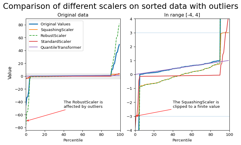
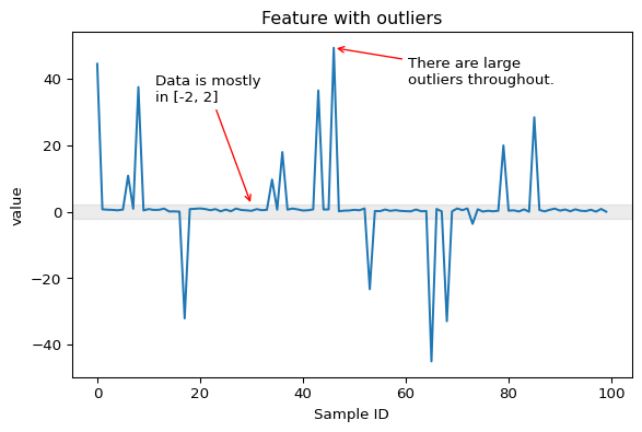
Encoding numerical features with `skrub.SquashingScaler`

Encoding categorical (string/text) features

Categorical features have a “cardinality”: the number of unique values

Low cardinality features: OneHotEncoder
High cardinality features (>40 unique values): skrub.StringEncoder
Textual features: skrub.TextEncoder and pretrained models from HuggingFace Hub

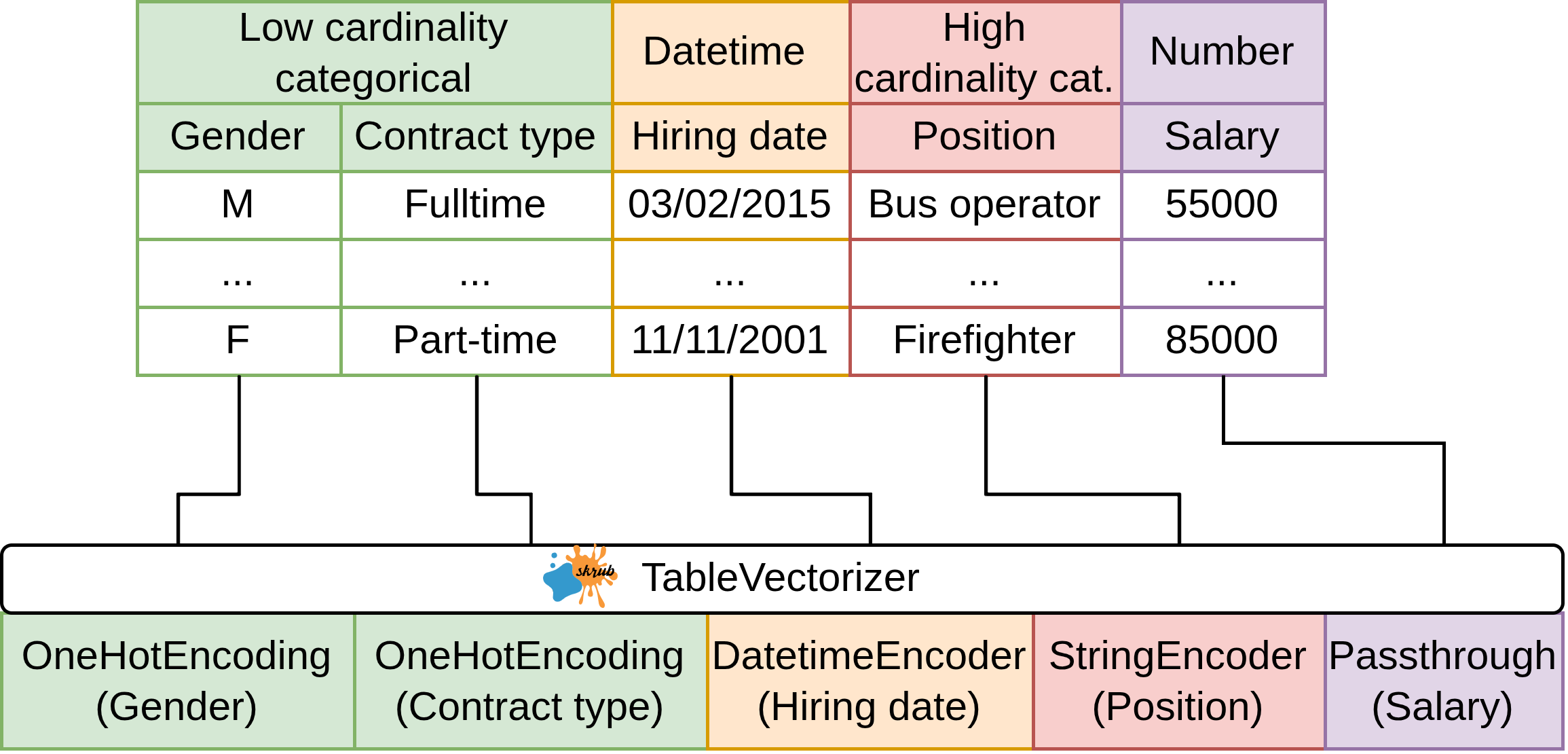
Encoding all the features: `TableVectorizer`

from skrub import TableVectorizer, TextEncoder

text = TextEncoder()
table_vec = TableVectorizer(high_cardinality=text)
df_encoded = table_vec.fit_transform(df)

Encoding all the features: `TableVectorizer`

Fine-grained column transformations with `ApplyToCols`

import pandas as pd
from sklearn.compose import make_column_selector as selector
from sklearn.compose import make_column_transformer
from sklearn.preprocessing import StandardScaler, OneHotEncoder

df = pd.DataFrame({"text": ["foo", "bar", "baz"], "number": [1, 2, 3]})

categorical_columns = selector(dtype_include=object)(df)
numerical_columns = selector(dtype_exclude=object)(df)

ct = make_column_transformer(
      (StandardScaler(),
       numerical_columns),
      (OneHotEncoder(handle_unknown="ignore"),
       categorical_columns))
transformed = ct.fit_transform(df)
transformed

array([[-1.22474487,  0.        ,  0.        ,  1.        ],
       [ 0.        ,  1.        ,  0.        ,  0.        ],
       [ 1.22474487,  0.        ,  1.        ,  0.        ]])

Fine-grained column transformations with `ApplyToCols`

import skrub.selectors as s
from sklearn.pipeline import make_pipeline
from skrub import ApplyToCols

numeric = ApplyToCols(StandardScaler(), cols=s.numeric())
string = ApplyToCols(OneHotEncoder(sparse_output=False), cols=s.string())

transformed = make_pipeline(numeric, string).fit_transform(df)
transformed

	text_bar	text_baz	text_foo	number
0	0.0	0.0	1.0	-1.224745
1	1.0	0.0	0.0	0.000000
2	0.0	1.0	0.0	1.224745

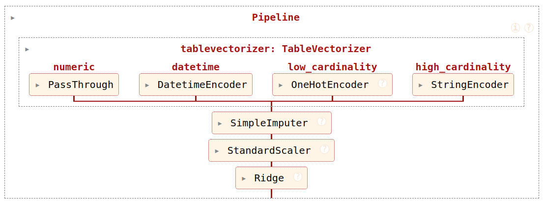
Build a predictive pipeline

from sklearn.linear_model import Ridge
model = Ridge()

Build a predictive pipeline

from sklearn.linear_model import Ridge
from sklearn.pipeline import make_pipeline
from sklearn.preprocessing import StandardScaler
from sklearn.impute import SimpleImputer

model = make_pipeline(StandardScaler(), SimpleImputer(), Ridge())

Build a predictive pipeline

from sklearn.linear_model import Ridge
from sklearn.pipeline import make_pipeline
from sklearn.preprocessing import StandardScaler, OneHotEncoder
from sklearn.impute import SimpleImputer
from sklearn.compose import make_column_selector as selector
from sklearn.compose import make_column_transformer

categorical_columns = selector(dtype_include=object)(employees)
numerical_columns = selector(dtype_exclude=object)(employees)

ct = make_column_transformer(
      (StandardScaler(),
       numerical_columns),
      (OneHotEncoder(handle_unknown="ignore"),
       categorical_columns))

model = make_pipeline(ct, SimpleImputer(), Ridge())

Build a predictive pipeline with `tabular_pipeline`

import skrub
from sklearn.linear_model import Ridge
model = skrub.tabular_pipeline(Ridge())

We now have a pipeline!

Gather some data
Explore the data
- skrub.TableReport
Pre-process the data
- Cleaner, ToDatetime …
Perform feature engineering
- skrub.TableVectorizer,SquashingScaler, TextEncoder, StringEncoder…
Build a scikit-learn pipeline
- tabular_pipeline, sklearn.pipeline.make_pipeline …
???
Profit 📈

What if this is not enough??

What if…

Your data is spread over multiple tables?
You want to avoid data leakage?
You want to tune more than just the hyperparameters of your model?
You want to guarantee that your pipeline is replayed exactly on new data?

When a normal pipe is not enough…

… the skrub DataOps come to the rescue 🚒

DataOps…

Extend the scikit-learn machinery to complex multi-table operations, and take care of data leakage
Track all operations with a computational graph (a Data Ops plan)
Allow tuning any operation in the data plan
Can be persisted and shared easily

How do DataOps work, though?

DataOps wrap around user operations, where user operations are:

any dataframe operation (e.g., merge, group by, aggregate etc.)
scikit-learn estimators (a Random Forest, RidgeCV etc.)
custom user code (load data from a path, fetch from an URL etc.)

Important

DataOps record user operations, so that they can later be replayed in the same order and with the same arguments on unseen data.

DataOps, Plans, `learner`s: oh my!

A DataOp (singular) wraps a single operation, and can be combined and concatenated with other DataOps.
The Data Ops Plan is a collective name for the directed computational graph that tracks a sequence and combination of DataOps.
The plan can be exported as a standalone object called learner. The learner works like a scikit-learn estimator that takes a dictionary of values rather than just X and y.

Starting with the `DataOps`

import skrub
data = skrub.datasets.fetch_credit_fraud()

baskets = skrub.var("baskets", data.baskets)
products = skrub.var("products", data.products) # add a new variable

X = baskets[["ID"]].skb.mark_as_X()
y = baskets["fraud_flag"].skb.mark_as_y()

X, y, products represent inputs to the pipeline.
skrub splits X and y when training.

Building a full data plan

from skrub import selectors as s

vectorizer = skrub.TableVectorizer(
    high_cardinality=skrub.StringEncoder()
)
vectorized_products = products.skb.apply(vectorizer, cols=s.all() - "basket_ID")

Building a full data plan

aggregated_products = vectorized_products.groupby(
    "basket_ID"
).agg("mean").reset_index()

features = X.merge(aggregated_products, left_on="ID", right_on="basket_ID")
features = features.drop(columns=["ID", "basket_ID"])

Building a full data plan

from sklearn.ensemble import ExtraTreesClassifier  
predictions = features.skb.apply(
    ExtraTreesClassifier(n_jobs=-1), y=y
)

Inspecting the data plan

predictions.skb.full_report()

Execution report

Each node:

Shows a preview of the data resulting from the operation
Reports the location in the code where the code is defined
Shows the run time of the node (in the next release)

Exporting the plan in a `learner`

The data plan can be exported as a learner:

# anywhere
learner = predictions.skb.make_learner(fitted=True)

Then, the learner can be pickled …

import pickle

with open("learner.bin", "wb") as fp:
    pickle.dump(learner, fp)

… loaded …

with open("learner.bin", "rb") as fp:
    loaded_learner = pickle.load(fp)

… and applied to new data:

data = skrub.datasets.fetch_credit_fraud(split="test")
new_baskets = data.baskets
new_products = data.products
loaded_learner.predict({"baskets": new_baskets, "products": new_products})

array([0, 0, 0, ..., 0, 0, 0], shape=(31549,))

Hyperparameter tuning in a Data Plan

skrub implements four choose_* functions:

choose_from: select from the given list of options
choose_int: select an integer within a range
choose_float: select a float within a range
choose_bool: select a bool
optional: chooses whether to execute the given operation

Tuning in `scikit-learn` can be complex

pipe = Pipeline([("dim_reduction", PCA()), ("regressor", Ridge())])
grid = [
    {
        "dim_reduction": [PCA()],
        "dim_reduction__n_components": [10, 20, 30],
        "regressor": [Ridge()],
        "regressor__alpha": loguniform(0.1, 10.0),
    },
    {
        "dim_reduction": [SelectKBest()],
        "dim_reduction__k": [10, 20, 30],
        "regressor": [Ridge()],
        "regressor__alpha": loguniform(0.1, 10.0),
    },
    {
        "dim_reduction": [PCA()],
        "dim_reduction__n_components": [10, 20, 30],
        "regressor": [RandomForestClassifier()],
        "regressor__n_estimators": loguniform(20, 200),
    },
    {
        "dim_reduction": [SelectKBest()],
        "dim_reduction__k": [10, 20, 30],
        "regressor": [RandomForestClassifier()],
        "regressor__n_estimators": loguniform(20, 200),
    },
]
model = RandomizedSearchCV(pipe, grid)

Tuning with `DataOps` is simple!

dim_reduction = X.skb.apply(
    skrub.choose_from(
        {
            "PCA": PCA(n_components=skrub.choose_int(10, 30)),
            "SelectKBest": SelectKBest(k=skrub.choose_int(10, 30))
        }, name="dim_reduction"
    )
)
regressor = dim_reduction.skb.apply(
    skrub.choose_from(
        {
            "Ridge": Ridge(alpha=skrub.choose_float(0.1, 10.0, log=True)),
            "RandomForest": RandomForestClassifier(
                n_estimators=skrub.choose_int(20, 200, log=True)
            )
        }, name="regressor"
    )
)
search = regressor.skb.make_randomized_search(scoring="roc_auc", fitted=True)

Tuning with `DataOps` is not limited to estimators

Pandas
Polars

df = pd.DataFrame(
    {"subject": ["math", "math", "art", "history"], "grade": [10, 8, 4, 6]}
)

df_do = skrub.var("grades", df)

agg_grades = df_do.groupby("subject").agg(skrub.choose_from(["count", "mean"]))
agg_grades.skb.describe_param_grid()

"- choose_from(['count', 'mean']): ['count', 'mean']\n"

df = pl.DataFrame(
    {"subject": ["math", "math", "art", "history"], "grade": [10, 8, 4, 6]}
)

df_do = skrub.var("grades", df)

agg_grades = df_do.group_by("subject").agg(
    skrub.choose_from([pl.mean("grade"), pl.count("grade")])
)
agg_grades.skb.describe_param_grid()

'- choose_from([<Expr [\'col("grade").mean()\'] at 0x783825B3A3D0>, <Expr [\'col("grade").count()\'] at 0x78382C9A0090>]): [<Expr [\'col("grade").mean()\'] at 0x783825B3A3D0>, <Expr [\'col("grade").count()\'] at 0x78382C9A0090>]\n'

Run hyperparameter search

# fit the search 
search = regressor.skb.make_randomized_search(scoring="roc_auc", fitted=True, cv=5)

# save the best learner
best_learner = search.best_learner_

Observe the impact of the hyperparameters

Data Ops provide a built-in parallel coordinate plot.

search = pred.skb.get_randomized_search(fitted=True)
search.plot_parallel_coord()

More information about the Data Ops

Skrub example gallery
Tutorial on timeseries forecasting at Euroscipy 2025
Skrub User guide
A Kaggle notebook on addressing the Titanic survival challenge with Data Ops

Wrapping up

Getting involved

Do you want to learn more?

Follow skrub on:

Star skrub on GitHub, or contribute directly:

Git repository

tl;dw

skrub provides

interactive data exploration
automated pre-processing of pandas and polars dataframes
powerful feature engineering
DataOps, plans, hyperparameter tuning, (almost) no leakage

EDF Talk: Skrub

Boost your productivity with skrub!

A teaser for later…

A teaser for later…

skrub compatibility

An example pipeline

Exploring the data

Exploring the data

Exploring the data with skrub

Data cleaning with pandas/polars: setup

Nulls, datetimes, constant columns with pandas/polars

Data cleaning with skrub.Cleaner

Comparison

Encoding datetime features with pandas/polars

Adding periodic features with pandas/polars

Encoding datetime features skrub.DatetimeEncoder

What periodic features look like

Encoding numerical features with skrub.SquashingScaler

Encoding numerical features with skrub.SquashingScaler

Encoding categorical (string/text) features

Encoding all the features: TableVectorizer

Encoding all the features: TableVectorizer

Fine-grained column transformations with ApplyToCols

Fine-grained column transformations with ApplyToCols

Build a predictive pipeline

Build a predictive pipeline

Build a predictive pipeline

Build a predictive pipeline with tabular_pipeline

We now have a pipeline!

What if this is not enough??

What if…

DataOps…

How do DataOps work, though?

DataOps, Plans, learners: oh my!

Starting with the DataOps

Building a full data plan

Building a full data plan

Building a full data plan

Inspecting the data plan

Exporting the plan in a learner

Hyperparameter tuning in a Data Plan

Tuning in scikit-learn can be complex

Tuning with DataOps is simple!

Tuning with DataOps is not limited to estimators

Run hyperparameter search

Observe the impact of the hyperparameters

More information about the Data Ops

Wrapping up

Getting involved

tl;dw

Exploring the data with `skrub`

Data cleaning with `skrub.Cleaner`

Encoding datetime features `skrub.DatetimeEncoder`

Encoding numerical features with `skrub.SquashingScaler`

Encoding numerical features with `skrub.SquashingScaler`

Encoding all the features: `TableVectorizer`

Encoding all the features: `TableVectorizer`

Fine-grained column transformations with `ApplyToCols`

Fine-grained column transformations with `ApplyToCols`

Build a predictive pipeline with `tabular_pipeline`

DataOps, Plans, `learner`s: oh my!

Starting with the `DataOps`

Exporting the plan in a `learner`

Tuning in `scikit-learn` can be complex

Tuning with `DataOps` is simple!

Tuning with `DataOps` is not limited to estimators