Data Preparation with skrub

A world without skrub

Let’s consider a world where skrub does not exist, and all we can do is use pandas and scikit-learn to prepare data for a machine learning model.

You may already be living in such a world.

Note

We want to build a simple model as baseline to decide whether there is enough of a signal in our data to build on.

Load and explore the data

import pandas as pd
import numpy as np

X = pd.read_csv("../data/employee_salaries/data.csv")
y = pd.read_csv("../data/employee_salaries/target.csv")["current_annual_salary"]
X.head(5)

	gender	department	department_name	division	assignment_category	employee_position_title	date_first_hired	year_first_hired
0	F	POL	Department of Police	MSB Information Mgmt and Tech Division Records...	Fulltime-Regular	Office Services Coordinator	09/22/1986	1986
1	M	POL	Department of Police	ISB Major Crimes Division Fugitive Section	Fulltime-Regular	Master Police Officer	09/12/1988	1988
2	F	HHS	Department of Health and Human Services	Adult Protective and Case Management Services	Fulltime-Regular	Social Worker IV	11/19/1989	1989
3	M	COR	Correction and Rehabilitation	PRRS Facility and Security	Fulltime-Regular	Resident Supervisor II	05/05/2014	2014
4	M	HCA	Department of Housing and Community Affairs	Affordable Housing Programs	Fulltime-Regular	Planning Specialist III	03/05/2007	2007

Explore the target

Let’s take a look at the target:

y.head(5)

0     69222.18
1     97392.47
2    104717.28
3     52734.57
4     93396.00
Name: current_annual_salary, dtype: float64

This is a regression task: we want to predict the value of current_annual_salary.

Strategizing

We can begin by exploring the dataframe with .describe, and then think of a plan for pre-processing our data.

X.describe(include="all")

	gender	department	department_name	division	assignment_category	employee_position_title	date_first_hired	year_first_hired
count	9211	9228	9228	9228	9228	9228	9228	9228.000000
unique	2	37	37	694	2	443	2264	NaN
top	M	POL	Department of Police	School Health Services	Fulltime-Regular	Bus Operator	12/12/2016	NaN
freq	5481	1844	1844	300	8394	638	87	NaN
mean	NaN	NaN	NaN	NaN	NaN	NaN	NaN	2003.597529
std	NaN	NaN	NaN	NaN	NaN	NaN	NaN	9.327078
min	NaN	NaN	NaN	NaN	NaN	NaN	NaN	1965.000000
25%	NaN	NaN	NaN	NaN	NaN	NaN	NaN	1998.000000
50%	NaN	NaN	NaN	NaN	NaN	NaN	NaN	2005.000000
75%	NaN	NaN	NaN	NaN	NaN	NaN	NaN	2012.000000
max	NaN	NaN	NaN	NaN	NaN	NaN	NaN	2016.000000

Our plan

We need to:

Impute some missing values in the gender column.
Encode convert categorical features into numerical features.
Convert the column date_first_hired into numerical features.
Scale numerical features (we’ll be using a linear model).
Evaluate the performance of the model.

Step 1: Convert date features to numerical

We extract numerical features from the date_first_hired column.

# Create a copy to work with
X_processed = X.copy()

# Parse the date column
X_processed['date_first_hired'] = pd.to_datetime(X_processed['date_first_hired'])

# Extract numerical features from date
X_processed['hired_month'] = X_processed['date_first_hired'].dt.month
X_processed['hired_year'] = X_processed['date_first_hired'].dt.year

# Drop original date column
X_processed = X_processed.drop('date_first_hired', axis=1)

print("Features after date transformation:")
print("\nShape:", X_processed.shape)

Features after date transformation:

Shape: (9228, 9)

Step 2: Encode categorical features

We encode the categorical features using one-hot encoding.

# Find the categorical columns
categorical_cols = X_processed.select_dtypes(include=['object']).columns.tolist()
print("Categorical columns to encode:", categorical_cols)

# Apply one-hot encoding only to categorical columns
X_encoded = pd.get_dummies(X_processed, columns=categorical_cols)
print("\nShape after encoding:", X_encoded.shape)

Categorical columns to encode: ['gender', 'department', 'department_name', 'division', 'assignment_category', 'employee_position_title']

Shape after encoding: (9228, 1218)

Step 3: Impute missing values

Some models cannot handle missing values.

We impute the missing values in the gender column:

from sklearn.impute import SimpleImputer

# Impute missing values with most frequent value
imputer = SimpleImputer(strategy='most_frequent')
X_encoded_imputed = pd.DataFrame(
    imputer.fit_transform(X_encoded),
    columns=X_encoded.columns
)

Step 3: Impute missing values

Important

Missing values are important! The fact that a value is missing is by itself useful information, and the pattern of missingness is also important.

For this reason, skrub transformers keep missing values as they are to retain the information content.

Example:

A dataset about employment has the column current position. A missing value here likely indicates unemployment, and imputing it with “most frequent” would lead to incorrect assumptions about the sample.

Step 4: Scale numerical features

Some models work better when all the numeric features have comparable scale.

RidgeCV is one of them, so we need to scale numerical features.

from sklearn.preprocessing import StandardScaler

# Initialize the scaler
scaler = StandardScaler()

# Fit and transform the data
X_scaled = scaler.fit_transform(X_encoded_imputed)
X_scaled = pd.DataFrame(X_scaled, columns=X_encoded_imputed.columns)

Warning

Outliers (values very far from the mean) make scaling hard to do. Robust scaling is needed.

Step 5: Train Ridge model with cross-validation

Train a RidgeCV regression model and evaluate with cross-validation.

from sklearn.linear_model import RidgeCV
from sklearn.model_selection import cross_val_score, cross_validate
import numpy as np

# Initialize Ridge model
ridge = RidgeCV()

# Perform cross-validation (5-fold)
cv_results = cross_validate(ridge, X_scaled, y, cv=5, scoring=["r2", "neg_mean_squared_error"])

# Convert MSE to RMSE
test_rmse = np.sqrt(-cv_results["test_neg_mean_squared_error"])

# Display results
print("Cross-Validation Results:")
print(
    f"Mean test R²: {cv_results['test_r2'].mean():.4f} (+/- {cv_results['test_r2'].std():.4f})"
)
print(f"Mean test RMSE: {test_rmse.mean():.4f} (+/- {test_rmse.std():.4f})")

Cross-Validation Results:
Mean test R²: 0.8731 (+/- 0.0276)
Mean test RMSE: 10329.8687 (+/- 1421.8752)

“Just ask an agent to write the code”

Operations in the wrong order.
Trying to impute categorical features without converting them to numeric values.
The datetime feature was treated like a categorical feature.
Cells could not be executed in order without proper debugging and re-prompting.
pd.get_dummies was executed on the full dataframe, rather than only on the training split, leading to data leakage.

Intermission: data leakage and fit/transform

from sklearn.impute import SimpleImputer

df = pd.DataFrame({
    "value": [1, 3, None, 5, 10, None, 1000, 5]
})

df_train = df[:5]
df_test = df[5:]

df_train

	value
0	1.0
1	3.0
2	NaN
3	5.0
4	10.0

df_test

	value
5	NaN
6	1000.0
7	5.0

Intermission: data leakage and fit/transform

What happens if you try to find the mean over all data?

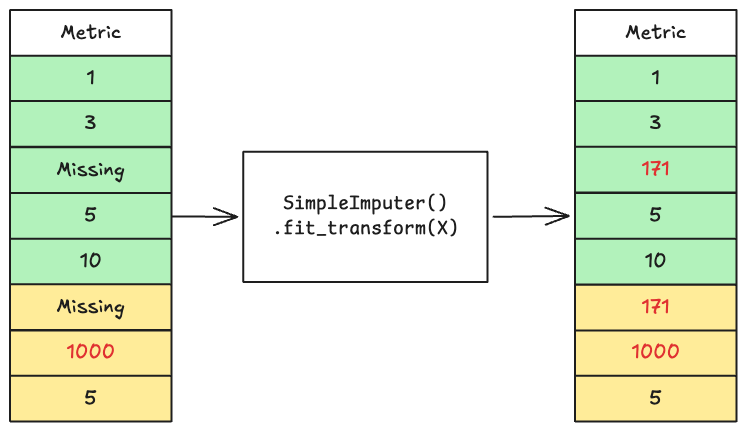
imputer = SimpleImputer(strategy="mean").set_output(transform="pandas")
df_imputed = imputer.fit_transform(df)

Intermission: data leakage and fit/transform

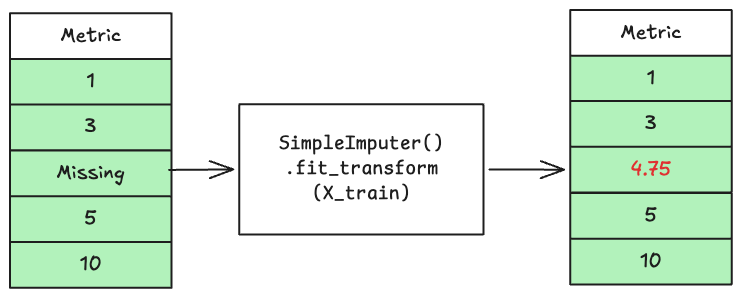
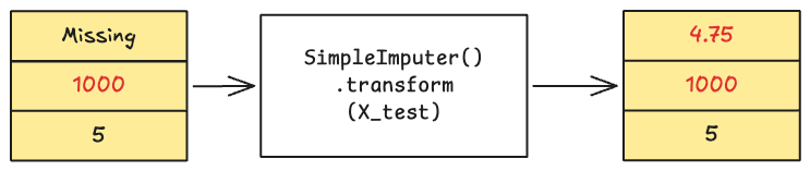
The proper way to do it: fit the transformer on the training data, transform the training with the same mean:

print(imputer.fit(df_train).transform(df_test))

Waking up from a nightmare

Thankfully, we can import skrub:

from skrub import tabular_pipeline

# Perform cross-validation (5-fold)
cv_results = cross_validate(tabular_pipeline("regression"), X, y, cv=5, 
                            scoring=['r2', 'neg_mean_squared_error'],
                            return_train_score=True)

# Convert MSE to RMSE
train_rmse = np.sqrt(-cv_results['train_neg_mean_squared_error'])
test_rmse = np.sqrt(-cv_results['test_neg_mean_squared_error'])

# Display results
print("Cross-Validation Results:")
print(f"Mean test R²: {cv_results['test_r2'].mean():.4f} (+/- {cv_results['test_r2'].std():.4f})")
print(f"Mean test RMSE: {test_rmse.mean():.4f} (+/- {test_rmse.std():.4f})")

Cross-Validation Results:
Mean test R²: 0.9105 (+/- 0.0145)
Mean test RMSE: 8696.1651 (+/- 973.8721)

What’s in the `tabular_pipeline`

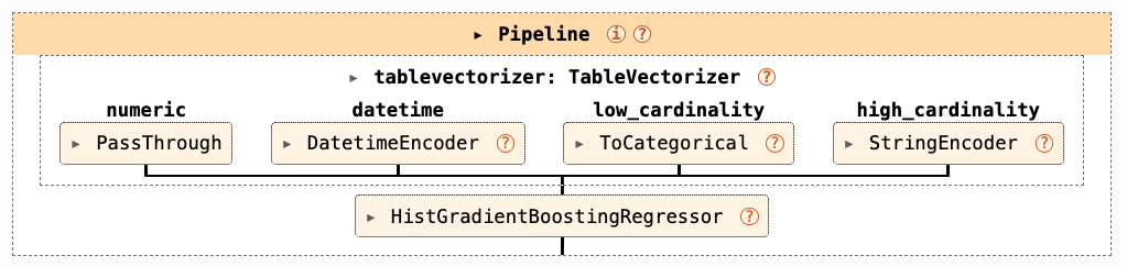
Pre-processing is part of the pipeline!

There isn’t a clear separation between “pre-processing”, “feature engineering” and “learning”.

If you learn something while pre-processing your training data (“this is a datetime”), you need to apply that knowledge to the test data.

This is why skrub provides transformers, rather than functions: transformers are stateful and can be used in pipelines, functions are not.

What we saw in this chapter

We built a predictive pipeline using traditional tools
We talked about missing data imputation
We discussed data leakage
We tested skrub’s tabular_pipeline
We covered why pre-processing is part of the pipeline

Course Roadmap

Data exploration with skrub’s TableReport
Data cleaning and sanitization with the Cleaner
Columnwise operations with ApplyToCols
Advanced column selectors and how to use them
Automatic feature engineering with the TableVectorizer
A robust baseline for machine learning tasks with the tabular_pipeline

If there is enough time:

Feature engineering with the skrub encoders

Data Preparation with skrub

A world without skrub

Load and explore the data

Explore the target

Strategizing

Our plan

Step 1: Convert date features to numerical

Step 2: Encode categorical features

Step 3: Impute missing values

Step 3: Impute missing values

Step 4: Scale numerical features

Step 5: Train Ridge model with cross-validation

“Just ask an agent to write the code”

Intermission: data leakage and fit/transform

Intermission: data leakage and fit/transform

Intermission: data leakage and fit/transform

Waking up from a nightmare

What’s in the tabular_pipeline

Pre-processing is part of the pipeline!

What we saw in this chapter

Course Roadmap

What’s in the `tabular_pipeline`