Exploring dataframes with skrub

Why do we need to explore data?

Before any kind of data processing or usage, we need to know what we are dealing with.

Useful information includes:

• The size of the dataset.
• The data types and names of the columns.
• How values are distributed in each column.
• Whether missing values are present, in what measure and where.
• Which features are discrete/categorical, and how many categories there are.
• Whether columns are strongly correlated with each other.

Loading the data

import pandas as pd
# Load the Adult Census dataset
data =  pd.read_csv("../data/adult_census/data.csv")
target =  pd.read_csv("../data/adult_census/target.csv")

Exploring data with Pandas tools 1/3

Let’s first explore the data using Pandas only.

data.head(5)

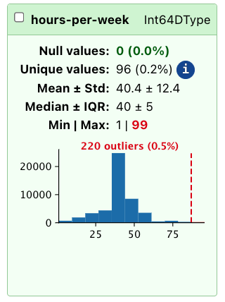
	age	workclass	fnlwgt	education	education-num	marital-status	occupation	relationship	race	sex	capital-gain	capital-loss	hours-per-week	native-country
0	25	Private	226802	11th	7	Never-married	Machine-op-inspct	Own-child	Black	Male	0	0	40	United-States
1	38	Private	89814	HS-grad	9	Married-civ-spouse	Farming-fishing	Husband	White	Male	0	0	50	United-States
2	28	Local-gov	336951	Assoc-acdm	12	Married-civ-spouse	Protective-serv	Husband	White	Male	0	0	40	United-States
3	44	Private	160323	Some-college	10	Married-civ-spouse	Machine-op-inspct	Husband	Black	Male	7688	0	40	United-States
4	18	NaN	103497	Some-college	10	Never-married	NaN	Own-child	White	Female	0	0	30	United-States

Exploring data with Pandas tools 2/3

If we want to have a simpler view of the datatypes in the dataframe, we must use data.info():

data.info()

<class 'pandas.core.frame.DataFrame'>
RangeIndex: 48842 entries, 0 to 48841
Data columns (total 14 columns):
 #   Column          Non-Null Count  Dtype 
---  ------          --------------  ----- 
 0   age             48842 non-null  int64 
 1   workclass       46043 non-null  object
 2   fnlwgt          48842 non-null  int64 
 3   education       48842 non-null  object
 4   education-num   48842 non-null  int64 
 5   marital-status  48842 non-null  object
 6   occupation      46033 non-null  object
 7   relationship    48842 non-null  object
 8   race            48842 non-null  object
 9   sex             48842 non-null  object
 10  capital-gain    48842 non-null  int64 
 11  capital-loss    48842 non-null  int64 
 12  hours-per-week  48842 non-null  int64 
 13  native-country  47985 non-null  object
dtypes: int64(6), object(8)
memory usage: 5.2+ MB

Exploring data with Pandas tools 3/3

We can also get a richer summary of the data with the .describe() method:

data.describe(include="all")

	age	workclass	fnlwgt	education	education-num	marital-status	occupation	relationship	race	sex	capital-gain	capital-loss	hours-per-week	native-country
count	48842.000000	46043	4.884200e+04	48842	48842.000000	48842	46033	48842	48842	48842	48842.000000	48842.000000	48842.000000	47985
unique	NaN	8	NaN	16	NaN	7	14	6	5	2	NaN	NaN	NaN	41
top	NaN	Private	NaN	HS-grad	NaN	Married-civ-spouse	Prof-specialty	Husband	White	Male	NaN	NaN	NaN	United-States
freq	NaN	33906	NaN	15784	NaN	22379	6172	19716	41762	32650	NaN	NaN	NaN	43832
mean	38.643585	NaN	1.896641e+05	NaN	10.078089	NaN	NaN	NaN	NaN	NaN	1079.067626	87.502314	40.422382	NaN
std	13.710510	NaN	1.056040e+05	NaN	2.570973	NaN	NaN	NaN	NaN	NaN	7452.019058	403.004552	12.391444	NaN
min	17.000000	NaN	1.228500e+04	NaN	1.000000	NaN	NaN	NaN	NaN	NaN	0.000000	0.000000	1.000000	NaN
25%	28.000000	NaN	1.175505e+05	NaN	9.000000	NaN	NaN	NaN	NaN	NaN	0.000000	0.000000	40.000000	NaN
50%	37.000000	NaN	1.781445e+05	NaN	10.000000	NaN	NaN	NaN	NaN	NaN	0.000000	0.000000	40.000000	NaN
75%	48.000000	NaN	2.376420e+05	NaN	12.000000	NaN	NaN	NaN	NaN	NaN	0.000000	0.000000	45.000000	NaN
max	90.000000	NaN	1.490400e+06	NaN	16.000000	NaN	NaN	NaN	NaN	NaN	99999.000000	4356.000000	99.000000	NaN

Exploring data with the TableReport

The TableReport computes various statistics about the given dataframe and presents them in an interactive format:

from skrub import TableReport
TableReport(data)

Ref

The Preview tab

The TableReport shows all the columns in the dataset, and allows to select and copy the content of the cells shown in the preview.

As this is a preview, only the first and last few rows are displayed.

The Stats tab

The Stats tab includes information about each column:

• full name
• detected dtype (no parsing!)
• presence of nulls
• cardinality (number of unique values)
• additional statistics for numerical features

The Distributions tab

A histogram is drawn for each column to show the distribution of values in that column.

Most frequent values are also displayed

The Associations tab

Cramer’s V and Pearson’s correlation coefficient are measured for all pairs of columns.

Associations show whether there are strong correlations between columns, and columns that may be redundant.

Outlier detection

The TableReport detects outliers using a simple interquartile test, marking as outliers all values that are beyond the IQR. This is a simple heuristic, and should not be treated as perfect. If your problem requires reliable outlier detection, you should not rely exclusively on what the TableReport shows.

Filtering the displayed columns

Pre-made column filters are also available, allowing to select columns by dtype or other characteristics. Filters are shared across tabs. It is also possible to define custom filters to select only specific columns:

my_filter = {"only_education": ["education", "education-num"]}

TableReport(data, column_filters=my_filter)

Please enable javascript

The skrub table reports need javascript to display correctly. If you are displaying a report in a Jupyter notebook and you see this message, you may need to re-execute the cell or to trust the notebook (button on the top right or "File > Trust notebook").

Skrub selectors can be used for that (more on that later).

Exploring the target variable

Besides dataframes, the TableReport handles series and mono- and bi-dimensional numpy arrays.

TableReport(target)

Please enable javascript

The skrub table reports need javascript to display correctly. If you are displaying a report in a Jupyter notebook and you see this message, you may need to re-execute the cell or to trust the notebook (button on the top right or "File > Trust notebook").

Working with big tables

Plot generation and computation of associations are very expensive operations, so it may be beneficial to disable them while working with very big tables.

Use the plot_distributions and compute_associations parameters to do so:

TableReport(
    data, plot_distributions=False, compute_associations=False, open_tab="distributions"
)

Please enable javascript

The skrub table reports need javascript to display correctly. If you are displaying a report in a Jupyter notebook and you see this message, you may need to re-execute the cell or to trust the notebook (button on the top right or "File > Trust notebook").

Exporting the TableReport

The TableReport computes many statistics about a given table. Typically, the interactive view is sufficient when developing with a notebook.

It is also possible to export the statistics in various formats to share them, or to use them programmatically.

Exporting the TableReport: HTML

The TableReport can be saved on disk as an HTML.

TableReport(data).write_html("report.html")

Tip

The report can be opened using any internet browser, with no need to run a Jupyter notebok or a python interactive console.

Exporting the TableReport: JSON

It is also possible to export the report in JSON format:

json_str = TableReport(data).json()

Important

If the report is generating distribution plots, the JSON will include them in SVG format. Distributions can be disabled by setting plot_distributions=False.

Exporting the TableReport: Markdown

(in the upcoming release!)

Finally, the report can be exported in summarized form as a Markdown-formatted string:

md_str = TableReport(data).markdown()

with open("report.md", "w") as fp:
    fp.write(md_str)

Warning

The TableReport does not do any sanitization of the input data, and prints out column names and most frequent values as part of the output. Do not feed the content of the report to an agent if the dataset is large, or if its content is not trusted.

What we have seen in this chapter

• Creating and configuring a TableReport for fast, interactive data exploration
• Exploring column statistics, value distributions, and associations visually
• Detecting nulls, outliers, and highly correlated columns at a glance
• Filtering columns by type or characteristics using built-in filters
• Adjusting TableReport settings for large datasets to optimize performance
• Saving and exporting reports as HTML, JSON, and Markdown files