Skrub

Machine learning with dataframes

Riccardo Cappuzzo

Inria P16

2025-11-21

`whoami`

I am a research engineer at Inria as part of the SODA team and the P16 project, and I am the lead developer of skrub
I’m Italian, but I don’t drink coffee, wine, and I like pizza with fries
I did my PhD in Côte d’Azur, and I moved away because it was too sunny and I don’t like the sea

Building a predictive pipeline with skrub

Premise and warning

Important

This lecture should give you an idea of possible problems you might run into, and how skrub can help you deal with (some of) them. The idea is giving you material you can refer back to if you encounter the same issue later on.

Skrub compatibility

Skrub is fully compatible with pandas and polars
Skrub transformers are fully compatible with scikit-learn

An example pipeline

Gather some data
Explore the data
Preprocess the data
Perform feature engineering
Build a scikit-learn pipeline
???
Profit?

Gathering the data: reading files, parsing dtypes

What happens if pandas parses this?

id,code,name,slug
15,76,Occitanie,occitanie
16,84,Auvergne-Rhône-Alpes,"auvergne rhone alpes"
17,93,"Provence-Alpes-Côte d'Azur","provence alpes cote dazur"
18,94,Corse,corse
19,COM,"Collectivités d'Outre-Mer","collectivites doutre mer"

What happens if pandas parses this?

import pandas as pd
pd.read_csv(file_path)

	id	code	name	slug
0	15	76	Occitanie	occitanie
1	16	84	Auvergne-Rhône-Alpes	auvergne rhone alpes
2	17	93	Provence-Alpes-Côte d'Azur	provence alpes cote dazur
3	18	94	Corse	corse
4	19	COM	Collectivités d'Outre-Mer	collectivites doutre mer

How about now?

Department code;Department name;Town code;Town name;Registered;Abstentions;Null;Choice A;Choice B
ZZ;FRANCAIS DE L'ETRANGER;8;Europe du Sud, Turquie, Israël;109763;84466;292;9299;15706
ZZ;FRANCAIS DE L'ETRANGER;9;Afrique Nord-Ouest;98997;59887;321;22116;16673
ZZ;FRANCAIS DE L'ETRANGER;10;Afrique Centre, Sud et Est;89859;46782;566;17008;25503
ZZ;FRANCAIS DE L'ETRANGER;11;Europe de l'est, Asie, Océanie;80061;42911;488;13975;22687

How about now?

import pandas as pd
pd.read_csv(file_path)

		Department code;Department name;Town code;Town name;Registered;Abstentions;Null;Choice A;Choice B
ZZ;FRANCAIS DE L'ETRANGER;8;Europe du Sud	Turquie	Israël;109763;84466;292;9299;15706
ZZ;FRANCAIS DE L'ETRANGER;9;Afrique Nord-Ouest;98997;59887;321;22116;16673	NaN	NaN
ZZ;FRANCAIS DE L'ETRANGER;10;Afrique Centre	Sud et Est;89859;46782;566;17008;25503	NaN
ZZ;FRANCAIS DE L'ETRANGER;11;Europe de l'est	Asie	Océanie;80061;42911;488;13975;22687

Parsing CSV files is difficult!

CSV files are plain text files and do not store any info besides what you can see.
Any information about dtypes is lost.
It is very hard to automate discovering the separator (ambiguity is unavoidable).
Files cannot be seeked: to get to a line, all the previous lines must be read first.
Plain text is uncompressed and can take up a very large amount of space.
Adding metadata is difficult and may make parsing harder.

CSV vs Parquet

Apache Parquet is a binary data storage format that addresses various issues with storing data.
Dtypes are well defined and fixed.
No separators to deal with: each column is defined in a schema when the parquet file is created.
Additional metadata can be stored to provide context to the data.
Parquet files are seekable: no need to read through the entire thing to get to a specific line.
Parquet files are compressed, reducing the size by multiple times (depending on data)
Parquet files are not human-readable. CSV files are, but are you really going to manually go through a few million lines of text?

Pandas vs Polars with Parquet

Pandas requires additional dependencies to read Parquet files (pyarrow or fastparquet).
Polars supports Parquet files natively and includes additional features that make use of the format.

Exploring the data

Exploratory analysis

Before starting any kind of training, it’s important to explore the data:

How big is the dataset (on disk, in rows/columns etc.)?
What kind of datatypes are we dealing with? Anything that needs more attention?
What is the distribution of values in a column?
Are there null values? In what columns?
Are there columns that may leak information to my model?
Are there columns that look problematic? (this takes experience)

This is not an exhaustive list!

Exploring the data with Pandas: parsing

import pandas as pd
import skrub
from skrub.datasets import fetch_employee_salaries

df = fetch_employee_salaries().X
df.head(5)

	gender	department	department_name	division	assignment_category	employee_position_title	date_first_hired	year_first_hired
0	F	POL	Department of Police	MSB Information Mgmt and Tech Division Records...	Fulltime-Regular	Office Services Coordinator	09/22/1986	1986
1	M	POL	Department of Police	ISB Major Crimes Division Fugitive Section	Fulltime-Regular	Master Police Officer	09/12/1988	1988
2	F	HHS	Department of Health and Human Services	Adult Protective and Case Management Services	Fulltime-Regular	Social Worker IV	11/19/1989	1989
3	M	COR	Correction and Rehabilitation	PRRS Facility and Security	Fulltime-Regular	Resident Supervisor II	05/05/2014	2014
4	M	HCA	Department of Housing and Community Affairs	Affordable Housing Programs	Fulltime-Regular	Planning Specialist III	03/05/2007	2007

Exploring the data: describe

df.describe(include="all")

	gender	department	department_name	division	assignment_category	employee_position_title	date_first_hired	year_first_hired
count	9211	9228	9228	9228	9228	9228	9228	9228.000000
unique	2	37	37	694	2	443	2264	NaN
top	M	POL	Department of Police	School Health Services	Fulltime-Regular	Bus Operator	12/12/2016	NaN
freq	5481	1844	1844	300	8394	638	87	NaN
mean	NaN	NaN	NaN	NaN	NaN	NaN	NaN	2003.597529
std	NaN	NaN	NaN	NaN	NaN	NaN	NaN	9.327078
min	NaN	NaN	NaN	NaN	NaN	NaN	NaN	1965.000000
25%	NaN	NaN	NaN	NaN	NaN	NaN	NaN	1998.000000
50%	NaN	NaN	NaN	NaN	NaN	NaN	NaN	2005.000000
75%	NaN	NaN	NaN	NaN	NaN	NaN	NaN	2012.000000
max	NaN	NaN	NaN	NaN	NaN	NaN	NaN	2016.000000

Exploring the data: column info

df.info()

<class 'pandas.core.frame.DataFrame'>
RangeIndex: 9228 entries, 0 to 9227
Data columns (total 8 columns):
 #   Column                   Non-Null Count  Dtype 
---  ------                   --------------  ----- 
 0   gender                   9211 non-null   object
 1   department               9228 non-null   object
 2   department_name          9228 non-null   object
 3   division                 9228 non-null   object
 4   assignment_category      9228 non-null   object
 5   employee_position_title  9228 non-null   object
 6   date_first_hired         9228 non-null   object
 7   year_first_hired         9228 non-null   int64 
dtypes: int64(1), object(7)
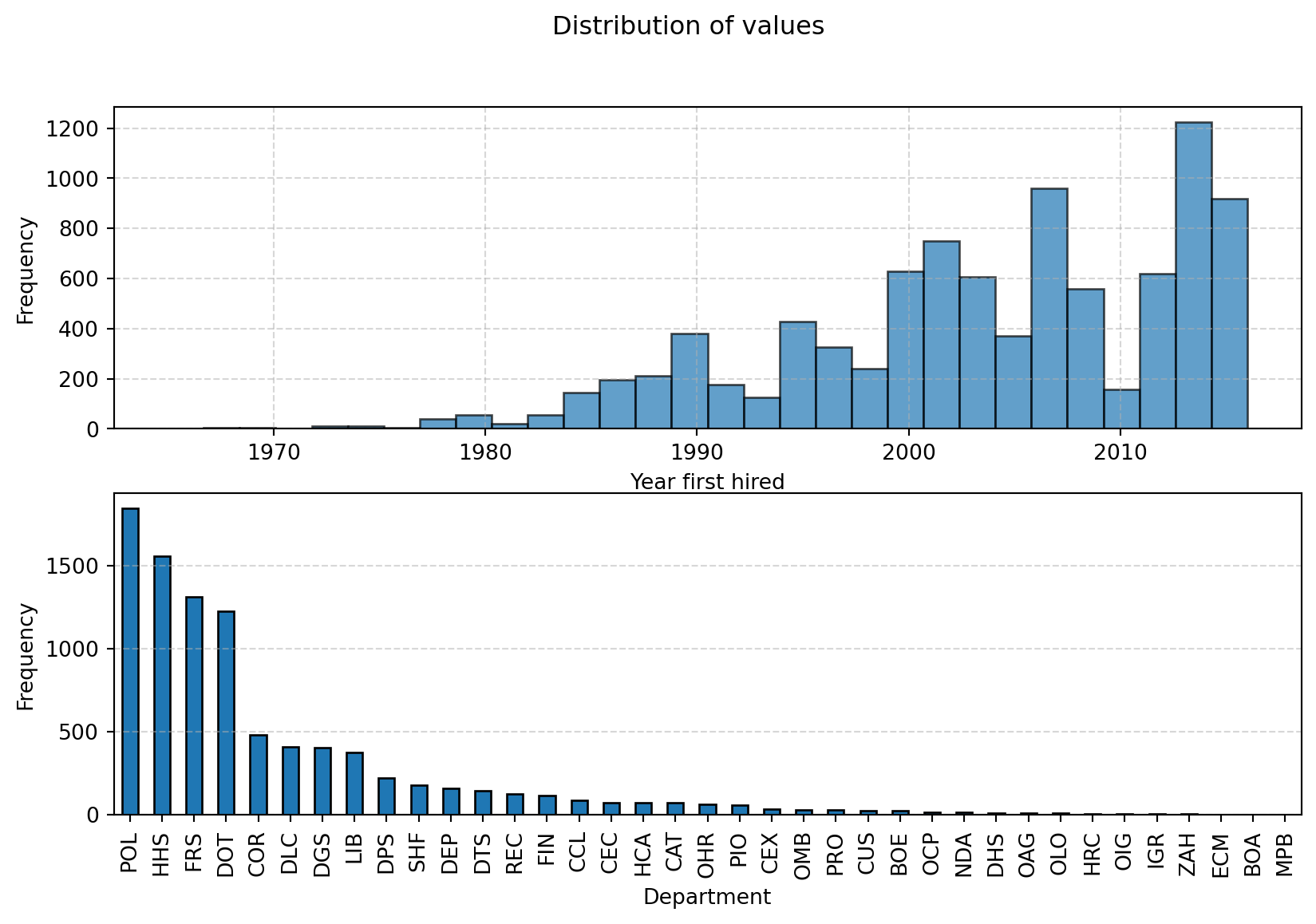
memory usage: 576.9+ KB

Exploring the data: distributions

import matplotlib.pyplot as plt
from pprint import pprint

# Plot the distribution of the numerical values using a histogram
fig, axs = plt.subplots(2,1, figsize=(10, 6))
ax1, ax2 = axs

ax1.hist(df['year_first_hired'], bins=30, edgecolor='black', alpha=0.7)
ax1.set_xlabel('Year first hired')
ax1.set_ylabel('Frequency')
ax1.grid(True, linestyle='--', alpha=0.5)

# Count the frequency of each category
category_counts = df['department'].value_counts()

# Create a bar plot
category_counts.plot(kind='bar', edgecolor='black', ax=ax2)

# Add labels and title
ax2.set_xlabel('Department')
ax2.set_ylabel('Frequency')
ax2.grid(True, linestyle='--', axis='y', alpha=0.5)  # Add grid lines for y-axis

fig.suptitle("Distribution of values")

# Show the plot
plt.show()

Exploring the data: distributions

Exploring the data with `skrub`

from skrub import TableReport
TableReport(employee_salaries)

TableReport Preview

Main features:

Obtain high-level statistics about the data
Explore the distribution of values and find outliers
Discover highly correlated columns
Export and share the report as an html file

More examples

Exploring the data with `skrub`

Things to notice:

Shape of the dataframe (rows, columns)
Dtype of the columns (string, numerical, datetime)
- Were dtypes converted properly?
Missing values
- Are there columns with many missing values?
Distribution of values
- Are there columns with high cardinality?
- Are there outliers?
- Are there columns with imbalanced distributions?
Column associations
- Are there correlated columns?

Pre-processing

import pandas as pd
import numpy as np

data = {
    "Int": [2, 3, 2],  # Multiple unique values
    "Const str": ["x", "x", "x"],  # Single unique value
    "Str": ["foo", "bar", "baz"],  # Multiple unique values
    "All nan": [np.nan, np.nan, np.nan],  # All missing values
    "All empty": ["", "", ""],  # All empty strings
    "Date": ["01 Jan 2023", "02 Jan 2023", "03 Jan 2023"],
}

df_pd = pd.DataFrame(data)
display(df_pd)

	Int	Const str	Str	All nan	Date
0	2	x	foo	NaN	01 Jan 2023
1	3	x	bar	NaN	02 Jan 2023
2	2	x	baz	NaN	03 Jan 2023

import polars as pl
import numpy as np
data = {
    "Int": [2, 3, 2],  # Multiple unique values
    "Const str": ["x", "x", "x"],  # Single unique value
    "Str": ["foo", "bar", "baz"],  # Multiple unique values
    "All nan": [np.nan, np.nan, np.nan],  # All missing values
    "All empty": ["", "", ""],  # All empty strings
    "Date": ["01 Jan 2023", "02 Jan 2023", "03 Jan 2023"],
}

df_pl = pl.DataFrame(data)
display(df_pl)

shape: (3, 6)

Int	Const str	Str	All nan	All empty	Date
i64	str	str	f64	str	str
2	"x"	"foo"	NaN	""	"01 Jan 2023"
3	"x"	"bar"	NaN	""	"02 Jan 2023"
2	"x"	"baz"	NaN	""	"03 Jan 2023"

Nulls, datetimes, constant columns with pandas/polars

Pandas
Polars

# Parse the datetime strings with a specific format
df_pd['Date'] = pd.to_datetime(df_pd['Date'], format='%d %b %Y')

# Drop columns with only a single unique value
df_pd_cleaned = df_pd.loc[:, df_pd.nunique(dropna=True) > 1]

# Function to drop columns with only missing values or empty strings
def drop_empty_columns(df):
    # Drop columns with only missing values
    df_cleaned = df.dropna(axis=1, how='all')
    # Drop columns with only empty strings
    empty_string_cols = df_cleaned.columns[df_cleaned.eq('').all()]
    df_cleaned = df_cleaned.drop(columns=empty_string_cols)
    return df_cleaned

# Apply the function to the DataFrame
df_pd_cleaned = drop_empty_columns(df_pd_cleaned)

# Parse the datetime strings with a specific format
df_pl = df_pl.with_columns([
    pl.col("Date").str.strptime(pl.Date, "%d %b %Y", strict=False).alias("Date")
])

# Drop columns with only a single unique value
df_pl_cleaned = df_pl.select([
    col for col in df_pl.columns if df_pl[col].n_unique() > 1
])

# Import selectors for dtype selection
import polars.selectors as cs

# Drop columns with only missing values or only empty strings
def drop_empty_columns(df):
    all_nan = df.select(
        [
            col for col in df.select(cs.numeric()).columns if 
            df [col].is_nan().all()
        ]
    ).columns
    
    all_empty = df.select(
        [
            col for col in df.select(cs.string()).columns if 
            (df[col].str.strip_chars().str.len_chars()==0).all()
        ]
    ).columns

    to_drop = all_nan + all_empty

    return df.drop(to_drop)

df_pl_cleaned = drop_empty_columns(df_pl_cleaned)

Data cleaning with `skrub.Cleaner`

Pandas
Polars

from skrub import Cleaner
cleaner = Cleaner(drop_if_constant=True, datetime_format='%d %b %Y')
df_cleaned = cleaner.fit_transform(df_pd)
display(df_cleaned)

	Int	Str	Date
0	2	foo	2023-01-01
1	3	bar	2023-01-02
2	2	baz	2023-01-03

from skrub import Cleaner
cleaner = Cleaner(drop_if_constant=True, datetime_format='%d %b %Y')
df_cleaned = cleaner.fit_transform(df_pl)
display(df_cleaned)

shape: (3, 3)

Int	Str	Date
i64	str	date
2	"foo"	2023-01-01
3	"bar"	2023-01-02
2	"baz"	2023-01-03

Cleaning `employee_salaries`

df = fetch_employee_salaries().X
df.info()

<class 'pandas.core.frame.DataFrame'>
RangeIndex: 9228 entries, 0 to 9227
Data columns (total 8 columns):
 #   Column                   Non-Null Count  Dtype 
---  ------                   --------------  ----- 
 0   gender                   9211 non-null   object
 1   department               9228 non-null   object
 2   department_name          9228 non-null   object
 3   division                 9228 non-null   object
 4   assignment_category      9228 non-null   object
 5   employee_position_title  9228 non-null   object
 6   date_first_hired         9228 non-null   object
 7   year_first_hired         9228 non-null   int64 
dtypes: int64(1), object(7)
memory usage: 576.9+ KB

Cleaning `employee_salaries`

cleaned = Cleaner().fit_transform(df)
cleaned.info()

<class 'pandas.core.frame.DataFrame'>
RangeIndex: 9228 entries, 0 to 9227
Data columns (total 8 columns):
 #   Column                   Non-Null Count  Dtype         
---  ------                   --------------  -----         
 0   gender                   9211 non-null   object        
 1   department               9228 non-null   object        
 2   department_name          9228 non-null   object        
 3   division                 9228 non-null   object        
 4   assignment_category      9228 non-null   object        
 5   employee_position_title  9228 non-null   object        
 6   date_first_hired         9228 non-null   datetime64[ns]
 7   year_first_hired         9228 non-null   int64         
dtypes: datetime64[ns](1), int64(1), object(6)
memory usage: 576.9+ KB

The `Cleaner`…

Automatically parses numerical values, even if they have string as dtype
Tries to parse datetimes, or takes a format from the user
Allows to drop uninformative columns:
- All nulls
- A single value
- All unique values (careful!)

Feature engineering

Encoding datetime features with pandas/polars

Pandas
Polars

import pandas as pd
data = {
    'date': ['2023-01-01 12:34:56', '2023-02-15 08:45:23', '2023-03-20 18:12:45'],
    'value': [10, 20, 30]
}
df_pd = pd.DataFrame(data)
datetime_column = "date"
df_pd[datetime_column] = pd.to_datetime(df_pd[datetime_column], errors='coerce')

df_pd['year'] = df_pd[datetime_column].dt.year
df_pd['month'] = df_pd[datetime_column].dt.month
df_pd['day'] = df_pd[datetime_column].dt.day
df_pd['hour'] = df_pd[datetime_column].dt.hour
df_pd['minute'] = df_pd[datetime_column].dt.minute
df_pd['second'] = df_pd[datetime_column].dt.second

import polars as pl
data = {
    'date': ['2023-01-01 12:34:56', '2023-02-15 08:45:23', '2023-03-20 18:12:45'],
    'value': [10, 20, 30]
}
df_pl = pl.DataFrame(data)
df_pl = df_pl.with_columns(date=pl.col("date").str.to_datetime())

df_pl = df_pl.with_columns(
    year=pl.col("date").dt.year(),
    month=pl.col("date").dt.month(),
    day=pl.col("date").dt.day(),
    hour=pl.col("date").dt.hour(),
    minute=pl.col("date").dt.minute(),
    second=pl.col("date").dt.second(),
)

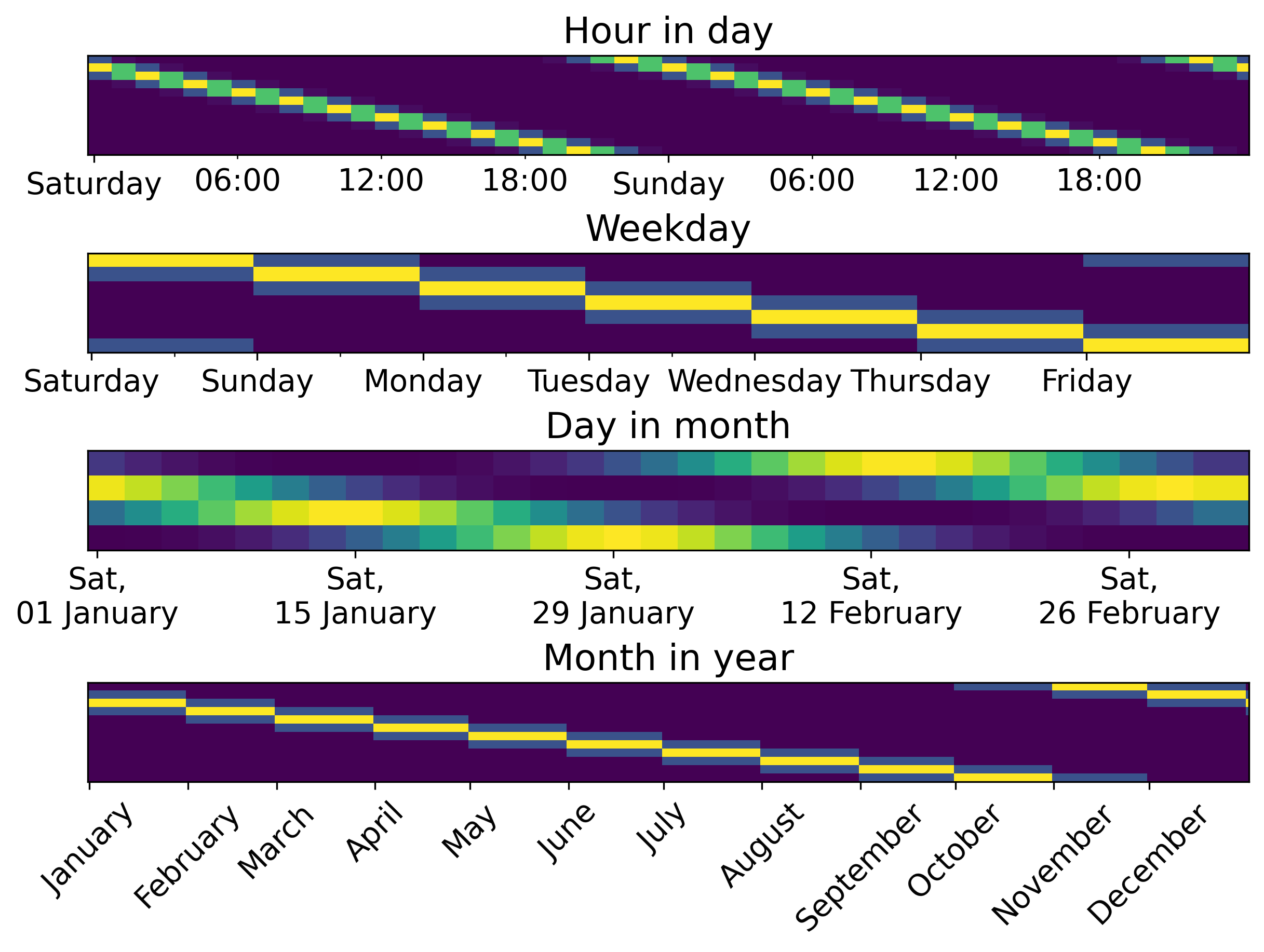
Adding periodic features with pandas/polars

Pandas
Polars

df_pd['hour_sin'] = np.sin(2 * np.pi * df_pd['hour'] / 24)
df_pd['hour_cos'] = np.cos(2 * np.pi * df_pd['hour'] / 24)

df_pd['month_sin'] = np.sin(2 * np.pi * df_pd['month'] / 12)
df_pd['month_cos'] = np.cos(2 * np.pi * df_pd['month'] / 12)

df_pl = df_pl.with_columns(
    hour_sin = np.sin(2 * np.pi * pl.col("hour") / 24),
    hour_cos = np.cos(2 * np.pi * pl.col("hour") / 24),
    
    month_sin = np.sin(2 * np.pi * pl.col("month") / 12),
    month_cos = np.cos(2 * np.pi * pl.col("month") / 12),
)

Encoding datetime features with `skrub.DatetimeEncoder`

from skrub import DatetimeEncoder, ToDatetime

X_date = ToDatetime().fit_transform(df["date"])
de = DatetimeEncoder(resolution="second")
# de = DatetimeEncoder(periodic_encoding="spline")
X_enc = de.fit_transform(X_date)
print(X_enc)

shape: (3, 7)
┌───────────┬────────────┬──────────┬───────────┬─────────────┬─────────────┬────────────────────┐
│ date_year ┆ date_month ┆ date_day ┆ date_hour ┆ date_minute ┆ date_second ┆ date_total_seconds │
│ ---       ┆ ---        ┆ ---      ┆ ---       ┆ ---         ┆ ---         ┆ ---                │
│ f32       ┆ f32        ┆ f32      ┆ f32       ┆ f32         ┆ f32         ┆ f32                │
╞═══════════╪════════════╪══════════╪═══════════╪═════════════╪═════════════╪════════════════════╡
│ 2023.0    ┆ 1.0        ┆ 1.0      ┆ 12.0      ┆ 34.0        ┆ 56.0        ┆ 1.6726e9           │
│ 2023.0    ┆ 2.0        ┆ 15.0     ┆ 8.0       ┆ 45.0        ┆ 23.0        ┆ 1.6765e9           │
│ 2023.0    ┆ 3.0        ┆ 20.0     ┆ 18.0      ┆ 12.0        ┆ 45.0        ┆ 1.6793e9           │
└───────────┴────────────┴──────────┴───────────┴─────────────┴─────────────┴────────────────────┘

Encoding datetime features `skrub.DatetimeEncoder`

from skrub import DatetimeEncoder, ToDatetime

X_date = ToDatetime().fit_transform(df["date"])
de = DatetimeEncoder(periodic_encoding="circular")
X_enc = de.fit_transform(X_date)
print(X_enc)

shape: (3, 8)
┌───────────┬────────────┬────────────┬────────────┬───────────┬───────────┬───────────┬───────────┐
│ date_year ┆ date_total ┆ date_month ┆ date_month ┆ date_day_ ┆ date_day_ ┆ date_hour ┆ date_hour │
│ ---       ┆ _seconds   ┆ _circular_ ┆ _circular_ ┆ circular_ ┆ circular_ ┆ _circular ┆ _circular │
│ f32       ┆ ---        ┆ 0          ┆ 1          ┆ 0         ┆ 1         ┆ _0        ┆ _1        │
│           ┆ f32        ┆ ---        ┆ ---        ┆ ---       ┆ ---       ┆ ---       ┆ ---       │
│           ┆            ┆ f64        ┆ f64        ┆ f64       ┆ f64       ┆ f64       ┆ f64       │
╞═══════════╪════════════╪════════════╪════════════╪═══════════╪═══════════╪═══════════╪═══════════╡
│ 2023.0    ┆ 1.6726e9   ┆ 0.5        ┆ 0.866025   ┆ 0.207912  ┆ 0.978148  ┆ 1.2246e-1 ┆ -1.0      │
│           ┆            ┆            ┆            ┆           ┆           ┆ 6         ┆           │
│ 2023.0    ┆ 1.6765e9   ┆ 0.866025   ┆ 0.5        ┆ 1.2246e-1 ┆ -1.0      ┆ 0.866025  ┆ -0.5      │
│           ┆            ┆            ┆            ┆ 6         ┆           ┆           ┆           │
│ 2023.0    ┆ 1.6793e9   ┆ 1.0        ┆ 6.1232e-17 ┆ -0.866025 ┆ -0.5      ┆ -1.0      ┆ -1.8370e- │
│           ┆            ┆            ┆            ┆           ┆           ┆           ┆ 16        │
└───────────┴────────────┴────────────┴────────────┴───────────┴───────────┴───────────┴───────────┘

What periodic features look like

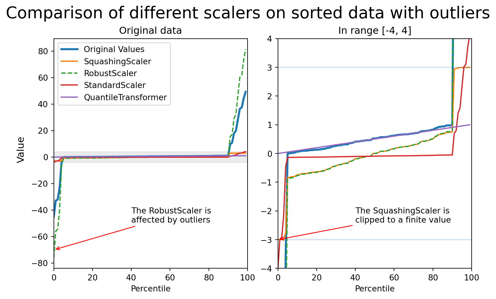
Scaling numerical features: outliers!

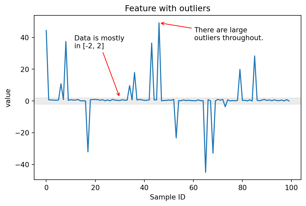
Comparing different scalers in presence of outliers

Dealing with categorical features

“Categorical features” include all features that belong to “discrete categories”.
For example, actual categories (grades, clothing sizes, countries…).
Text is also categorical! Any unique string is a category.
There may be many unique categories.

How do you deal with that?

Basic strategies: `OneHotEncoder`

The OneHotEncoder creates an indicator column for each unique value in a column.
Fine if you have few categories, problematic if you have many.

from sklearn.preprocessing import OneHotEncoder

df = fetch_employee_salaries().X
enc = OneHotEncoder(sparse_output=False).fit_transform(X=df[["gender"]])

print("The number of unique values in column `gender` is: ", df[["gender"]].nunique().item())
print("The shape of the OneHotEncoding of column `gender` is: ", enc.shape)

The number of unique values in column `gender` is:  2
The shape of the OneHotEncoding of column `gender` is:  (9228, 3)

Looks fine!

Basic strategies: `OneHotEncoder`

What about a different column?

enc = OneHotEncoder(sparse_output=False).fit_transform(X=df[["division"]])

print("The number of unique values in column `division` is: ", df[["division"]].nunique().item())
print("The shape of the OneHotEncoding of column `division` is: ", enc.shape)

The number of unique values in column `division` is:  694
The shape of the OneHotEncoding of column `division` is:  (9228, 694)

Warning

That’s ~700 features that are mostly 0’s.

Remember that more features mean:

Overfitting
Worse performance
Increased training time and resources needed
Worse interpretability

Basic strategies: `OrdinalEncoder`

from sklearn.preprocessing import OrdinalEncoder

enc = OrdinalEncoder().fit_transform(X=df[["division"]])

print("The number of unique values in column `division` is: ", df[["division"]].nunique().item())
print("The shape of the OneHotEncoding of column `division` is: ", enc.shape)

The number of unique values in column `division` is:  694
The shape of the OneHotEncoding of column `division` is:  (9228, 1)

Now we’re keeping the number of dimensions down, but we are introducing an ordering that may not make any sense in reality.

Encoding categorical (string/text) features

Categorical features have a “cardinality”: the number of unique values

Low cardinality features: OneHotEncoder.
- The OneHotEncoder produces sparse matrices. Dataframes are dense.
High cardinality features (>40 unique values):
- Using OneHotEncoder generates too many (dense) features.
- Use encoders with a fixed number of output features.
Latent Semantic Analysis with: skrub.StringEncoder
- Apply tf-idf to the ngrams in the column, followed by SVD.
- Robust, quick, fixed number of output features regardless of # of unique values.

Encoding categorical (string/text) features

Textual features: skrub.TextEncoder and pretrained models from HuggingFace Hub.
- The TextEncoder needs PyTorch: very heavy dependency.
- Models are large and take time to download.
- Encoding is much slower.
- However, performance can be much better depending on the dataset.

Deeper dive in this post.

Building pipelines

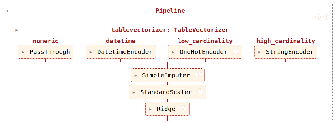
Encoding all the features: `TableVectorizer`

from skrub import TableVectorizer

table_vec = TableVectorizer()
df_encoded = table_vec.fit_transform(df)

Apply the Cleaner to all columns
Split columns by dtype and # of unique values
Encode each column separately

Encoding all the features: `TableVectorizer`

Fine-grained column transformations

Various skrub transformers can accept a cols parameter that lets you select what columns should be modified.
SelectCols, DropCols, ApplyToCols, ApplyToFrame, and .skb.apply() can take cols as a parameter.
Complex selection rules can be implemented with skrub.selectors.

Why is column selection important?

There is an index I don’t want to touch
Column names give me information about the content
I want to transform only datetimes (or numbers, or strings…)
I need to combine conditions (column has nulls AND column is numeric)

Selecting columns with the skrub selectors

import pandas as pd
from skrub import SelectCols
import skrub.selectors as s
df = pd.DataFrame(
    {
        "height_mm": [297.0, 420.0],
        "width_mm": [210.0, 297.0],
        "kind": ["A4", "A3"],
        "ID": [4, 3],
    }
)
SelectCols(cols=s.all()).fit_transform(df)

	height_mm	width_mm	kind	ID
0	297.0	210.0	A4	4
1	420.0	297.0	A3	3

Selecting columns with the skrub selectors

Select all columns based on the name:

SelectCols(s.glob('*_mm')).fit_transform(df)

	height_mm	width_mm
0	297.0	210.0
1	420.0	297.0

Select columns based on dtypes, and invert selections:

SelectCols(~s.numeric()).fit_transform(df)

	kind
0	A4
1	A3

More info in the selectors user guide.

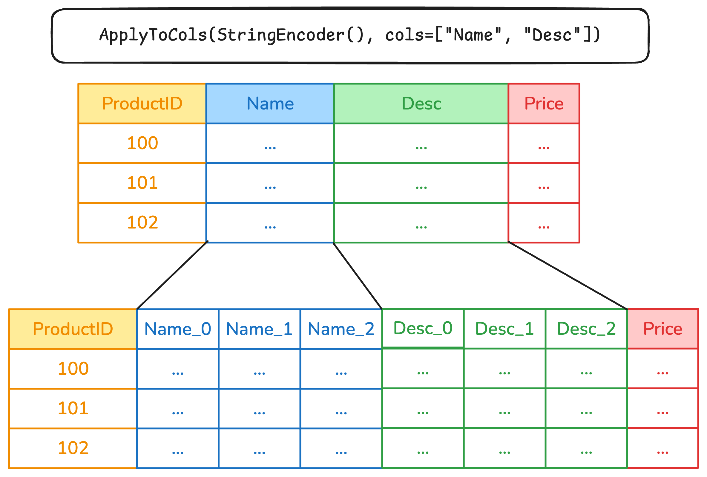
Column transformations with `ApplyToCols` and `ApplyToFrame`

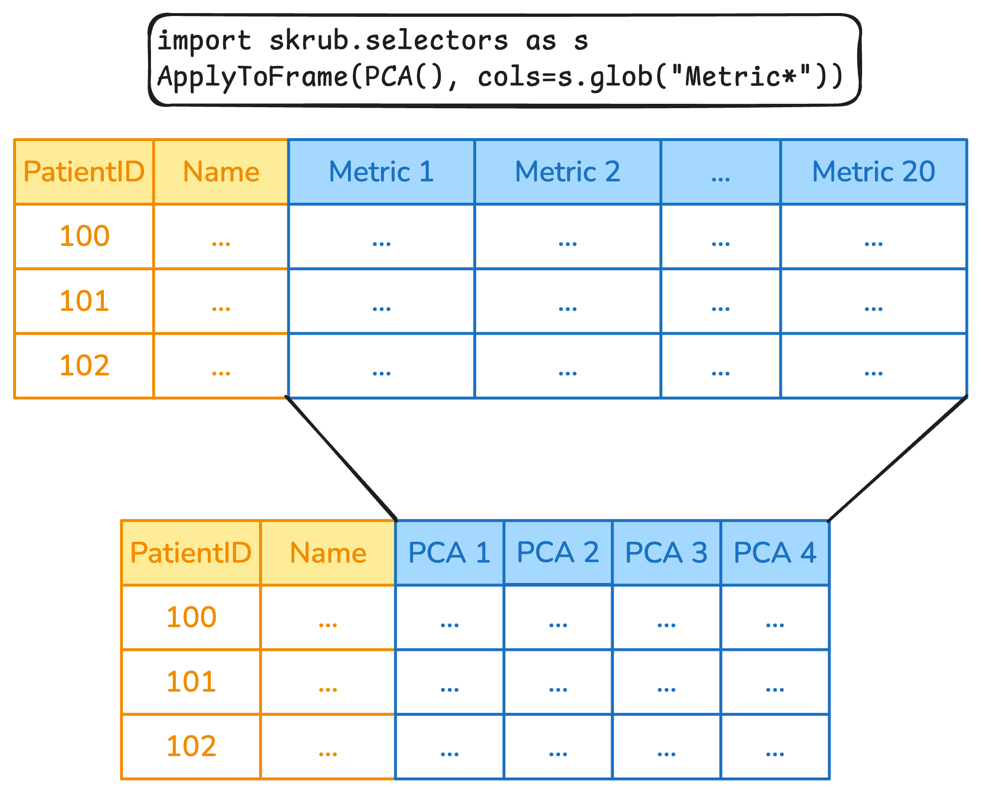
Replacing `ColumnTransformer` with `ApplyToCols`

import pandas as pd
from sklearn.compose import make_column_selector as selector
from sklearn.compose import make_column_transformer
from sklearn.preprocessing import StandardScaler, OneHotEncoder

df = pd.DataFrame({"text": ["foo", "bar", "baz"], "number": [1, 2, 3]})

categorical_columns = selector(dtype_include=object)(df)
numerical_columns = selector(dtype_exclude=object)(df)

ct = make_column_transformer(
      (StandardScaler(),
       numerical_columns),
      (OneHotEncoder(handle_unknown="ignore"),
       categorical_columns))
transformed = ct.fit_transform(df)
transformed

array([[-1.22474487,  0.        ,  0.        ,  1.        ],
       [ 0.        ,  1.        ,  0.        ,  0.        ],
       [ 1.22474487,  0.        ,  1.        ,  0.        ]])

Replacing `ColumnTransformer` with `ApplyToCols`

import skrub.selectors as s
from sklearn.pipeline import make_pipeline
from skrub import ApplyToCols

numeric = ApplyToCols(StandardScaler(), cols=s.numeric())
string = ApplyToCols(OneHotEncoder(sparse_output=False), cols=s.string())

transformed = make_pipeline(numeric, string).fit_transform(df)
transformed

	text_bar	text_baz	text_foo	number
0	0.0	0.0	1.0	-1.224745
1	1.0	0.0	0.0	0.000000
2	0.0	1.0	0.0	1.224745

Let’s build a predictive pipeline

from sklearn.linear_model import Ridge
model = Ridge()

Let’s build a predictive pipeline

from sklearn.linear_model import Ridge
from sklearn.pipeline import make_pipeline
from sklearn.preprocessing import StandardScaler
from sklearn.impute import SimpleImputer

model = make_pipeline(StandardScaler(), SimpleImputer(), Ridge())

Let’s build a predictive pipeline

from sklearn.linear_model import Ridge
from sklearn.pipeline import make_pipeline
from sklearn.preprocessing import StandardScaler, OneHotEncoder
from sklearn.impute import SimpleImputer
from sklearn.compose import make_column_selector as selector
from sklearn.compose import make_column_transformer

categorical_columns = selector(dtype_include=object)(employees)
numerical_columns = selector(dtype_exclude=object)(employees)

ct = make_column_transformer(
      (StandardScaler(),
       numerical_columns),
      (OneHotEncoder(handle_unknown="ignore"),
       categorical_columns))

model = make_pipeline(ct, SimpleImputer(), Ridge())

Now with `tabular_pipeline`

import skrub
from sklearn.linear_model import Ridge
model = skrub.tabular_pipeline(Ridge())

We now have a pipeline!

Gather some data
Explore the data
- TableReport
Pre-process the data
- Cleaner …
Perform feature engineering
- TableVectorizer, SquashingScaler, TextEncoder, StringEncoder…
Build a scikit-learn pipeline
- tabular_pipeline, sklearn.pipeline.make_pipeline …
???
Profit 📈

Skrub Data Ops

Disclaimer

Warning

This section covers more advanced topics that are more representative of what happens in real scenarios, and how skrub can help addressing some of them.

What if…

Your data is spread over multiple tables?
You want to avoid data leakage?
You want to tune more than just the hyperparameters of your model?
You want to guarantee that your pipeline is replayed exactly on new data?

When a normal pipeline is not enough…

… the skrub DataOps come to the rescue 🚒

DataOps…

Extend the scikit-learn machinery to complex multi-table operations.
Take care of data leakage.
Track all operations with a computational graph (a Data Ops plan).
Allow tuning any operation in the Data Ops plan.
Can be persisted and shared easily.

How do DataOps work, though?

DataOps wrap around user operations, where user operations are:

any dataframe operation (e.g., merge, group by, aggregate etc.).
scikit-learn estimators (a Random Forest, RidgeCV etc.).
custom user code (load data from a path, fetch from an URL etc.).

Important

DataOps record user operations, so that they can later be replayed in the same order and with the same arguments on unseen data.

Looking at the computational graph

predictions.skb.full_report()

Execution report

Each node:

Shows a preview of the data resulting from the operation
Reports the location in the code where the code is defined
Shows the run time of the node
Offline and in HTML, no need for a running kernel

Tuning in `scikit-learn` can be complex

pipe = Pipeline([("dim_reduction", PCA()), ("regressor", Ridge())])
grid = [
    {
        "dim_reduction": [PCA()],
        "dim_reduction__n_components": [10, 20, 30],
        "regressor": [Ridge()],
        "regressor__alpha": loguniform(0.1, 10.0),
    },
    {
        "dim_reduction": [SelectKBest()],
        "dim_reduction__k": [10, 20, 30],
        "regressor": [Ridge()],
        "regressor__alpha": loguniform(0.1, 10.0),
    },
    {
        "dim_reduction": [PCA()],
        "dim_reduction__n_components": [10, 20, 30],
        "regressor": [RandomForestRegressor()],
        "regressor__n_estimators": loguniform(20, 200),
    },
    {
        "dim_reduction": [SelectKBest()],
        "dim_reduction__k": [10, 20, 30],
        "regressor": [RandomForestRegressor()],
        "regressor__n_estimators": loguniform(20, 200),
    },
]
model = RandomizedSearchCV(pipe, grid)

Tuning with `DataOps` is simple!

dim_reduction = X.skb.apply(
    skrub.choose_from(
        {
            "PCA": PCA(n_components=skrub.choose_int(10, 30)),
            "SelectKBest": SelectKBest(k=skrub.choose_int(10, 30))
        }, name="dim_reduction"
    )
)
regressor = dim_reduction.skb.apply(
    skrub.choose_from(
        {
            "Ridge": Ridge(alpha=skrub.choose_float(0.1, 10.0, log=True)),
            "RandomForest": RandomForestRegressor(
                n_estimators=skrub.choose_int(20, 200, log=True)
            )
        }, name="regressor"
    )
)
search = regressor.skb.make_randomized_search(scoring="roc_auc", fitted=True)

Run hyperparameter search

# fit the search 
search = regressor.skb.make_randomized_search(scoring="roc_auc", fitted=True, cv=5)

# save the best learner
best_learner = search.best_learner_

Hyperparameter tuning with `choose_*`

skrub implements four choose_* functions:

choose_from: select from the given list of options
choose_int: select an integer within a range
choose_float: select a float within a range
choose_bool: select a bool
optional: chooses whether to execute the given operation

Tuning with `DataOps` is not limited to estimators

Pandas
Polars

df = pd.DataFrame(
    {"subject": ["math", "math", "art", "history"], "grade": [10, 8, 4, 6]}
)

df_do = skrub.var("grades", df)

agg_grades = df_do.groupby("subject").agg(skrub.choose_from(["count", "mean", "max"]))
agg_grades.skb.describe_param_grid()

"- choose_from(['count', 'mean', 'max']): ['count', 'mean', 'max']\n"

df = pl.DataFrame(
    {"subject": ["math", "math", "art", "history"], "grade": [10, 8, 4, 6]}
)

df_do = skrub.var("grades", df)

agg_grades = df_do.group_by("subject").agg(
    skrub.choose_from([pl.mean("grade"), pl.count("grade")])
)
agg_grades.skb.describe_param_grid()

'- choose_from([<Expr [\'col("grade").mean()\'] at 0x354194A50>, <Expr [\'col("grade").count()\'] at 0x354194B50>]): [<Expr [\'col("grade").mean()\'] at 0x354194A50>, <Expr [\'col("grade").count()\'] at 0x354194B50>]\n'

How does tuning affect the results?

Data Ops provide a built-in parallel coordinate plot.

search = pred.skb.get_randomized_search(fitted=True)
search.plot_parallel_coord()

Exporting the plan in a `learner`

The Learner is a stand-alone object that works like a scikit-learn estimator that takes a dictionary as input rather than just X and y.

learner = predictions.skb.make_learner(fitted=True)

Then, the learner can be pickled …

import pickle

with open("learner.bin", "wb") as fp:
    pickle.dump(learner, fp)

… loaded and applied to new data:

with open("learner.bin", "rb") as fp:
    loaded_learner = pickle.load(fp)
data = skrub.datasets.fetch_credit_fraud(split="test")
new_baskets = data.baskets
new_products = data.products
loaded_learner.predict({"baskets": new_baskets, "products": new_products})

More information about Data Ops

Skrub example gallery
Tutorial on timeseries forecasting at Euroscipy 2025
Skrub User guide
A Kaggle notebook on addressing the Titanic survival challenge with Data Ops

Wrapping up

Getting involved

Do you want to learn more?

Follow skrub on:

Star skrub on GitHub, or contribute directly:

Git repository

tl;dw

skrub provides

interactive data exploration
automated pre-processing of pandas and polars dataframes
powerful feature engineering
DataOps, plans, hyperparameter tuning, (almost) no leakage

Skrub

whoami

Building a predictive pipeline with skrub

Premise and warning

Skrub compatibility

An example pipeline

Gathering the data: reading files, parsing dtypes

What happens if pandas parses this?

What happens if pandas parses this?

How about now?

How about now?

Parsing CSV files is difficult!

CSV vs Parquet

Pandas vs Polars with Parquet

Exploring the data

Exploratory analysis

Exploring the data with Pandas: parsing

Exploring the data: describe

Exploring the data: column info

Exploring the data: distributions

Exploring the data: distributions

Exploring the data with skrub

Exploring the data with skrub

Pre-processing

Data cleaning with pandas/polars: setup

Nulls, datetimes, constant columns with pandas/polars

Data cleaning with skrub.Cleaner

Cleaning employee_salaries

Cleaning employee_salaries

The Cleaner…

Feature engineering

Encoding datetime features with pandas/polars

Adding periodic features with pandas/polars

Encoding datetime features with skrub.DatetimeEncoder

Encoding datetime features skrub.DatetimeEncoder

What periodic features look like

Scaling numerical features: outliers!

Comparing different scalers in presence of outliers

Dealing with categorical features

Basic strategies: OneHotEncoder

Basic strategies: OneHotEncoder

Basic strategies: OrdinalEncoder

Encoding categorical (string/text) features

Encoding categorical (string/text) features

Building pipelines

Encoding all the features: TableVectorizer

Encoding all the features: TableVectorizer

Fine-grained column transformations

Why is column selection important?

Selecting columns with the skrub selectors

Selecting columns with the skrub selectors

Column transformations with ApplyToCols and ApplyToFrame

Column transformations with ApplyToCols and ApplyToFrame

Replacing ColumnTransformer with ApplyToCols

Replacing ColumnTransformer with ApplyToCols

Let’s build a predictive pipeline

Let’s build a predictive pipeline

Let’s build a predictive pipeline

Now with tabular_pipeline

We now have a pipeline!

Skrub Data Ops

Disclaimer

What if…

DataOps…

How do DataOps work, though?

Looking at the computational graph

Tuning in scikit-learn can be complex

Tuning with DataOps is simple!

Run hyperparameter search

Hyperparameter tuning with choose_*

Tuning with DataOps is not limited to estimators

How does tuning affect the results?

Exporting the plan in a learner

More information about Data Ops

Wrapping up

Getting involved

tl;dw

`whoami`

Exploring the data with `skrub`

Exploring the data with `skrub`

Data cleaning with `skrub.Cleaner`

Cleaning `employee_salaries`

Cleaning `employee_salaries`

The `Cleaner`…

Encoding datetime features with `skrub.DatetimeEncoder`

Encoding datetime features `skrub.DatetimeEncoder`

Basic strategies: `OneHotEncoder`

Basic strategies: `OneHotEncoder`

Basic strategies: `OrdinalEncoder`

Encoding all the features: `TableVectorizer`

Encoding all the features: `TableVectorizer`

Column transformations with `ApplyToCols` and `ApplyToFrame`

Column transformations with `ApplyToCols` and `ApplyToFrame`

Replacing `ColumnTransformer` with `ApplyToCols`

Replacing `ColumnTransformer` with `ApplyToCols`

Now with `tabular_pipeline`

Tuning in `scikit-learn` can be complex

Tuning with `DataOps` is simple!

Hyperparameter tuning with `choose_*`

Tuning with `DataOps` is not limited to estimators

Exporting the plan in a `learner`