
Note
Go to the end to download the full example code. or to run this example in your browser via JupyterLite or Binder
Fuzzy joining dirty tables with the Joiner#
Here we show how to combine data from different sources, with a vocabulary not well normalized.
Joining is difficult: one entry on one side does not have an exact match on the other side.
The fuzzy_join() function enables to join tables without cleaning the data by
accounting for the label variations.
To illustrate, we will join data from the 2022 World Happiness Report, with tables provided in the World Bank open data platform in order to create a first prediction model.
Moreover, the Joiner() is a scikit-learn Transformer that makes it easy to
use such fuzzy joining multiple tables to bring in information in a
machine-learning pipeline. In particular, it enables tuning parameters of
fuzzy_join() to find the matches that maximize prediction accuracy.
Data Importing and preprocessing#
We import the happiness score table first:
from skrub import datasets

happiness_data = datasets.fetch_country_happiness()
df = happiness_data.happiness_report
Downloading 'country_happiness' from https://github.com/skrub-data/skrub-data-files/raw/refs/heads/main/country_happiness.zip (attempt 1/3)
Let’s look at the table:
df.head(3)
This is a table that contains the happiness index of a country along with some of the possible explanatory factors: GDP per capita, Social support, Generosity etc.
For the sake of this example, we only keep the country names and our variable of interest: the ‘Happiness score’.
Additional tables from other sources#
Now, we need to include explanatory factors from other sources, to complete our covariates (X table).
Interesting tables can be found on the World Bank open data platform, which are also available in the dataset We extract the table containing GDP per capita by country:
Then another table, with life expectancy by country:
And a table with legal rights strength by country:
A correspondence problem#
Alas, the entries for countries do not perfectly match between our original table (df), and those that we downloaded from the worldbank (gdp_per_capita):
df.sort_values(by="Country").tail(7)
gdp_per_capita.sort_values(by="Country Name").tail(7)
We can see that Yemen is written “Yemen*” on one side, and “Yemen, Rep.” on the other.
We also have entries that probably do not have correspondences: “World” on one side, whereas the other table only has country-level data.
Joining tables with imperfect correspondence#
We will now join our initial table, df, with the 3 additional ones that we have extracted.
1. Joining GDP per capita table#
To join them with skrub, we only need to do the following:
from skrub import fuzzy_join

augmented_df = fuzzy_join(
    df,  # our table to join
    gdp_per_capita,  # the table to join with
    left_on="Country",  # the first join key column
    right_on="Country Name",  # the second join key column
    add_match_info=True,
)

augmented_df.tail(20)

# We merged the first World Bank table to our initial one.
We see that our fuzzy_join() successfully identified the countries,
even though some country names differ between tables.
For instance, “Egypt” and “Egypt, Arab Rep.” are correctly matched, as are “Lesotho*” and “Lesotho”.
Let’s do some more inspection of the merging done.
Let’s print the worst matches, which will give us an overview of the situation:
augmented_df.sort_values("skrub_Joiner_rescaled_distance").tail(10)
We see that some matches were unsuccessful (e.g “Palestinian Territories*” and “Palau”), because there is simply no match in the two tables.
In this case, it is better to use the threshold parameter (max_dist)
so as to include only precise-enough matches:
augmented_df = fuzzy_join(
    df,
    gdp_per_capita,
    left_on="Country",
    right_on="Country Name",
    max_dist=0.9,
    add_match_info=True,
)
augmented_df.sort_values("skrub_Joiner_rescaled_distance", ascending=False).head()
Matches that are not available (or precise enough) are marked as NaN.
We will remove them using the drop_unmatched parameter:
augmented_df = fuzzy_join(
    df,
    gdp_per_capita,
    left_on="Country",
    right_on="Country Name",
    drop_unmatched=True,
    max_dist=0.9,
    add_match_info=True,
)

augmented_df.drop(columns=["Country Name"], inplace=True)
We can finally plot and look at the link between GDP per capital and happiness:
import matplotlib.pyplot as plt
import seaborn as sns

sns.set_context("notebook")

plt.figure(figsize=(4, 3))
ax = sns.regplot(
    data=augmented_df,
    x="GDP per capita (current US$)",
    y="Happiness score",
    lowess=True,
)
ax.set_ylabel("Happiness index")
ax.set_title("Is a higher GDP per capita linked to happiness?")
plt.tight_layout()
plt.show()
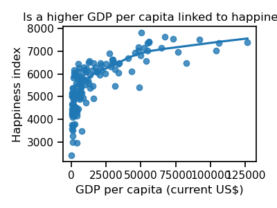
It seems that the happiest countries are those having a high GDP per capita. However, unhappy countries do not have only low levels of GDP per capita. We have to search for other patterns.
2. Joining life expectancy table#
Now let’s include other information that may be relevant, such as in the life_exp table:
augmented_df = fuzzy_join(
    augmented_df,
    life_exp,
    left_on="Country",
    right_on="Country Name",
    max_dist=0.9,
    add_match_info=True,
)

augmented_df.drop(columns=["Country Name"], inplace=True)

augmented_df.head(3)
Let’s plot this relation:
plt.figure(figsize=(4, 3))
fig = sns.regplot(
    data=augmented_df,
    x="Life expectancy at birth, total (years)",
    y="Happiness score",
    lowess=True,
)
fig.set_ylabel("Happiness index")
fig.set_title("Is a higher life expectancy linked to happiness?")
plt.tight_layout()
plt.show()
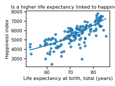
It seems the answer is yes! Countries with higher life expectancy are also happier.
3. Joining legal rights strength table#
And the table with a measure of legal rights strength in the country:
augmented_df = fuzzy_join(
    augmented_df,
    legal_rights,
    left_on="Country",
    right_on="Country Name",
    max_dist=0.9,
    add_match_info=True,
)

augmented_df.drop(columns=["Country Name"], inplace=True)

augmented_df.head(3)
Let’s take a look at their correspondence in a figure:
plt.figure(figsize=(4, 3))
fig = sns.regplot(
    data=augmented_df,
    x="Strength of legal rights index (0=weak to 12=strong)",
    y="Happiness score",
    lowess=True,
)
fig.set_ylabel("Happiness index")
fig.set_title("Does a country's legal rights strength lead to happiness?")
plt.tight_layout()
plt.show()
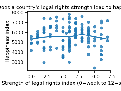
From this plot, it is not clear that this measure of legal strength is linked to happiness.
Great! Our joined table has become bigger and full of useful information. And now we are ready to apply a first machine learning model to it!
Prediction model#
We now separate our covariates (X), from the target (or exogenous) variables: y.
y = augmented_df["Happiness score"]
X = augmented_df.drop(["Happiness score", "Country"], axis=1)
Let us now define the model that will be used to predict the happiness score:
from sklearn.ensemble import HistGradientBoostingRegressor
from sklearn.model_selection import KFold

hgdb = HistGradientBoostingRegressor(random_state=0)
cv = KFold(n_splits=5, shuffle=True, random_state=0)
To evaluate our model, we will apply a 5-fold cross-validation. We evaluate our model using the R2 score.
Let’s finally assess the results of our models:
from sklearn.model_selection import cross_validate

cv_results_t = cross_validate(hgdb, X, y, cv=cv, scoring="r2")

cv_r2_t = cv_results_t["test_score"]

print(f"Mean R² score is {cv_r2_t.mean():.2f} +- {cv_r2_t.std():.2f}")
Mean R² score is 0.65 +- 0.08
We have a satisfying first result: an R² of 0.63!
Data cleaning varies from dataset to dataset: there are as
many ways to clean a table as there are errors. The fuzzy_join()
method is generalizable across all datasets.
Data transformation is also often very costly in both time and resources.
fuzzy_join() is fast and easy-to-use.
Now up to you, try improving our model by adding information into it and beating our result!
Using the Joiner() to fuzzy join multiple tables#
A convenient way to merge different tables from the World Bank
to X in a scikit-learn Pipeline and tune the parameters is to use the Joiner().
The Joiner() is a transformer that can fuzzy-join a table on
a main table.
Instantiating the transformer#
y = df["Happiness score"]
df = df.drop("Happiness score", axis=1)

from sklearn.pipeline import make_pipeline

from skrub import Joiner, SelectCols

# We create a selector that we will insert at the end of our pipeline, to
# select the relevant columns before fitting the regressor
selector = SelectCols(
    [
        "GDP per capita (current US$) gdp",
        "Life expectancy at birth, total (years) life_exp",
        "Strength of legal rights index (0=weak to 12=strong) legal_rights",
    ]
)

# And we can now put together the pipeline
pipeline = make_pipeline(
    Joiner(gdp_per_capita, main_key="Country", aux_key="Country Name", suffix=" gdp"),
    Joiner(life_exp, main_key="Country", aux_key="Country Name", suffix=" life_exp"),
    Joiner(
        legal_rights, main_key="Country", aux_key="Country Name", suffix=" legal_rights"
    ),
    selector,
    HistGradientBoostingRegressor(),
)
And the best part is that we are now able to evaluate the parameters of the fuzzy_join().
For instance, the match_score was manually picked and can now be
introduced into a grid search:
from sklearn.model_selection import GridSearchCV

# We will test 2 possible values of max_dist:
params = {
    "joiner-1__max_dist": [0.1, 0.9],
    "joiner-2__max_dist": [0.1, 0.9],
    "joiner-3__max_dist": [0.1, 0.9],
}

grid = GridSearchCV(pipeline, param_grid=params, cv=cv)
grid.fit(df, y)

print("Best parameters:", grid.best_params_)
Best parameters: {'joiner-1__max_dist': 0.1, 'joiner-2__max_dist': 0.9, 'joiner-3__max_dist': 0.1}
Total running time of the script: (0 minutes 14.591 seconds)