
Note
Go to the end to download the full example code. or to run this example in your browser via JupyterLite or Binder
Encoding: from a dataframe to a numerical matrix for machine learning#
This example shows how to transform a rich dataframe with columns of various types into a numerical matrix on which machine-learning algorithms can be applied. We study the case of predicting wages using the employee salaries dataset.
Easy learning on a dataframe#
Let’s first retrieve the dataset, using one of the downloaders from the
skrub.datasets module. As all the downloaders,
fetch_employee_salaries() returns a dataset with attributes
X, and y. X is a dataframe which contains the features (aka design matrix,
explanatory variables, independent variables). y is a column (pandas Series) which
contains the target (aka dependent, response variable) that we want to learn to
predict from X. In this case y is the annual salary.
from skrub.datasets import fetch_employee_salaries

dataset = fetch_employee_salaries()
employees, salaries = dataset.X, dataset.y
employees
Most machine-learning algorithms work with arrays of numbers. The
challenge here is that the employees dataframe is a heterogeneous
set of columns: some are numerical ('year_first_hired'), some dates
('date_first_hired'), some have a few categorical entries
('gender'), some many ('employee_position_title'). Therefore
our table needs to be “vectorized”: processed to extract numeric
features.
skrub provides an easy way to build a simple but reliable
machine-learning model which includes this step, working well on most
tabular data.
from sklearn.model_selection import cross_validate

from skrub import tabular_pipeline

model = tabular_pipeline("regressor")
results = cross_validate(model, employees, salaries)
results["test_score"]
array([0.91004969, 0.88245204, 0.91464581, 0.92346467, 0.92418526])
The estimator returned by tabular_pipeline combines 2 steps:
a
TableVectorizerto preprocess the dataframe and vectorize the featuresa supervised learner (by default a
HistGradientBoostingRegressor)
In the rest of this example, we focus on the first step and explore the
capabilities of skrub’s TableVectorizer.
More details on encoding tabular data#
from skrub import TableVectorizer

vectorizer = TableVectorizer()
vectorized_employees = vectorizer.fit_transform(employees)
vectorized_employees
From our 8 columns, the TableVectorizer has extracted 143 numerical
features. Most of them are one-hot encoded representations of the categorical
features. For example, we can see that 3 columns 'gender_F', 'gender_M',
'gender_nan' were created to encode the 'gender' column.
By performing appropriate transformations on our complex data, the TableVectorizer
produced numeric features that we can use for machine-learning:
from sklearn.ensemble import HistGradientBoostingRegressor

HistGradientBoostingRegressor().fit(vectorized_employees, salaries)
The TableVectorizer bridges the gap between tabular data and machine-learning
pipelines. It allows us to apply a machine-learning estimator to our dataframe without
manual data wrangling and feature extraction.
Inspecting the TableVectorizer#
The TableVectorizer distinguishes between 4 basic kinds of columns (more may be
added in the future).
For each kind, it applies a different transformation, which we can configure. The
kinds of columns and the default transformation for each of them are:
numeric columns: simply casting to floating-point
datetime columns: extracting features such as year, day, hour with the
DatetimeEncoderlow-cardinality categorical columns: one-hot encoding
high-cardinality categorical columns: a simple and effective text representation pipeline provided by the
GapEncoder
We can inspect which transformation was chosen for a each column and retrieve the
fitted transformer. vectorizer.kind_to_columns_ provides an overview of how the
vectorizer categorized columns in our input:
{'numeric': ['year_first_hired'], 'datetime': ['date_first_hired'], 'low_cardinality': ['gender', 'department', 'department_name', 'assignment_category'], 'high_cardinality': ['division', 'employee_position_title'], 'specific': []}
The reverse mapping is given by:
{'year_first_hired': 'numeric', 'date_first_hired': 'datetime', 'gender': 'low_cardinality', 'department': 'low_cardinality', 'department_name': 'low_cardinality', 'assignment_category': 'low_cardinality', 'division': 'high_cardinality', 'employee_position_title': 'high_cardinality'}
vectorizer.transformers_ gives us a dictionary which maps column names to the
corresponding transformer.
vectorizer.transformers_["date_first_hired"]
We can also see which features in the vectorizer’s output were derived from a given input column.
vectorizer.input_to_outputs_["date_first_hired"]
['date_first_hired_year', 'date_first_hired_month', 'date_first_hired_day', 'date_first_hired_total_seconds']
vectorized_employees[vectorizer.input_to_outputs_["date_first_hired"]]
Finally, we can go in the opposite direction: given a column in the input, find out from which input column it was derived.
vectorizer.output_to_input_["department_BOA"]
'department'
Dataframe preprocessing#
Note that "date_first_hired" has been recognized and processed as a datetime
column.
vectorizer.column_to_kind_["date_first_hired"]
'datetime'
But looking closer at our original dataframe, it was encoded as a string.
employees["date_first_hired"]
0       09/22/1986
1       09/12/1988
2       11/19/1989
3       05/05/2014
4       03/05/2007
           ...
9223    11/03/2015
9224    11/28/1988
9225    04/30/2001
9226    09/05/2006
9227    01/30/2012
Name: date_first_hired, Length: 9228, dtype: object
Note the dtype: object in the output above.
Before applying the transformers we specify, the TableVectorizer performs a few
preprocessing steps.
For example, strings commonly used to represent missing values such as "N/A" are
replaced with actual null. As we saw above, columns containing strings that
represent dates (e.g. '2024-05-15') are detected and converted to proper
datetimes.
We can inspect the list of steps that were applied to a given column:
vectorizer.all_processing_steps_["date_first_hired"]
[CleanNullStrings(), DropUninformative(), ToDatetime(), DatetimeEncoder(), {'date_first_hired_day': ToFloat32(), 'date_first_hired_month': ToFloat32(), ...}]
These preprocessing steps depend on the column:
vectorizer.all_processing_steps_["department"]
[CleanNullStrings(), DropUninformative(), ToStr(), OneHotEncoder(drop='if_binary', dtype='float32', handle_unknown='ignore',
              sparse_output=False), {'department_BOA': ToFloat32(), 'department_BOE': ToFloat32(), ...}]
A simple Pipeline for tabular data#
The TableVectorizer outputs data that can be understood by a scikit-learn
estimator. Therefore we can easily build a 2-step scikit-learn Pipeline
that we can fit, test or cross-validate and that works well on tabular data.
import numpy as np
from sklearn.ensemble import HistGradientBoostingRegressor
from sklearn.model_selection import cross_validate
from sklearn.pipeline import make_pipeline

pipeline = make_pipeline(TableVectorizer(), HistGradientBoostingRegressor())

results = cross_validate(pipeline, employees, salaries)
scores = results["test_score"]
print(f"R2 score:  mean: {np.mean(scores):.3f}; std: {np.std(scores):.3f}")
print(f"mean fit time: {np.mean(results['fit_time']):.3f} seconds")
R2 score:  mean: 0.912; std: 0.016
mean fit time: 2.307 seconds
Specializing the TableVectorizer for HistGradientBoosting#
The encoders used by default by the TableVectorizer are safe choices for a wide
range of downstream estimators. If we know we want to use it with a HistGradientBoostingRegressor (or
classifier) model, we can make some different choices that are only well-suited for
tree-based models but can yield a faster pipeline.
We make 2 changes.
The HistGradientBoostingRegressor has built-in support for categorical features, so we do not need to one-hot
encode them.
We do need to tell it which features should be treated as categorical with the
categorical_features parameter. In recent versions of scikit-learn, we can set
categorical_features='from_dtype', and it will treat all columns in the input that
have a Categorical dtype as such. Therefore we change the encoder for
low-cardinality columns: instead of OneHotEncoder, we use skrub’s
ToCategorical. This transformer will simply ensure our columns have an actual
Categorical dtype (as opposed to string for example), so that they can be
recognized by the HistGradientBoostingRegressor.
The second change replaces the GapEncoder with a MinHashEncoder.
The GapEncoder is a topic model.
It produces interpretable embeddings in a vector space where distances are meaningful,
which is great for interpretation and necessary for some downstream supervised
learners such as linear models. However fitting the topic model is costly in
computation time and memory. The MinHashEncoder produces features that are not easy
to interpret, but that decision trees can efficiently use to test for the occurrence
of particular character n-grams (more details are provided in its documentation).
Therefore it can be a faster and very effective alternative, when the supervised
learner is built on top of decision trees, which is the case for the HistGradientBoostingRegressor.
The resulting pipeline is identical to the one produced by default by
tabular_pipeline.
from skrub import MinHashEncoder, ToCategorical

vectorizer = TableVectorizer(
    low_cardinality=ToCategorical(), high_cardinality=MinHashEncoder()
)
pipeline = make_pipeline(
    vectorizer, HistGradientBoostingRegressor(categorical_features="from_dtype")
)

results = cross_validate(pipeline, employees, salaries)
scores = results["test_score"]
print(f"R2 score:  mean: {np.mean(scores):.3f}; std: {np.std(scores):.3f}")
print(f"mean fit time: {np.mean(results['fit_time']):.3f} seconds")
R2 score:  mean: 0.911; std: 0.014
mean fit time: 1.284 seconds
We can see that this new pipeline achieves a similar score but is fitted much faster.
This is mostly due to replacing GapEncoder with MinHashEncoder (however this makes
the features less interpretable).
Feature importances in the statistical model#
As we just saw, we can fit a MinHashEncoder faster than a GapEncoder. However, the
GapEncoder has a crucial advantage: each dimension of its output space is associated
with a topic which can be inspected and interpreted.
In this section, after training a regressor, we will plot the feature importances.
First, we train another scikit-learn regressor, the RandomForestRegressor:
from sklearn.ensemble import RandomForestRegressor

vectorizer = TableVectorizer()  # now using the default GapEncoder
regressor = RandomForestRegressor(n_estimators=50, max_depth=20, random_state=0)

pipeline = make_pipeline(vectorizer, regressor)
pipeline.fit(employees, salaries)
We are retrieving the feature importances:
avg_importances = regressor.feature_importances_
std_importances = np.std(
    [tree.feature_importances_ for tree in regressor.estimators_], axis=0
)
indices = np.argsort(avg_importances)[::-1]
And plotting the results:
import matplotlib.pyplot as plt

top_indices = indices[:20]
labels = vectorizer.get_feature_names_out()[top_indices]

plt.figure(figsize=(12, 9))
plt.barh(
    y=labels,
    width=avg_importances[top_indices],
    xerr=std_importances[top_indices],
    ecolor="k",
    color="b",
    alpha=0.5,
)
plt.yticks(fontsize=15)
plt.title("Feature importances")
plt.tight_layout(pad=1)
plt.show()
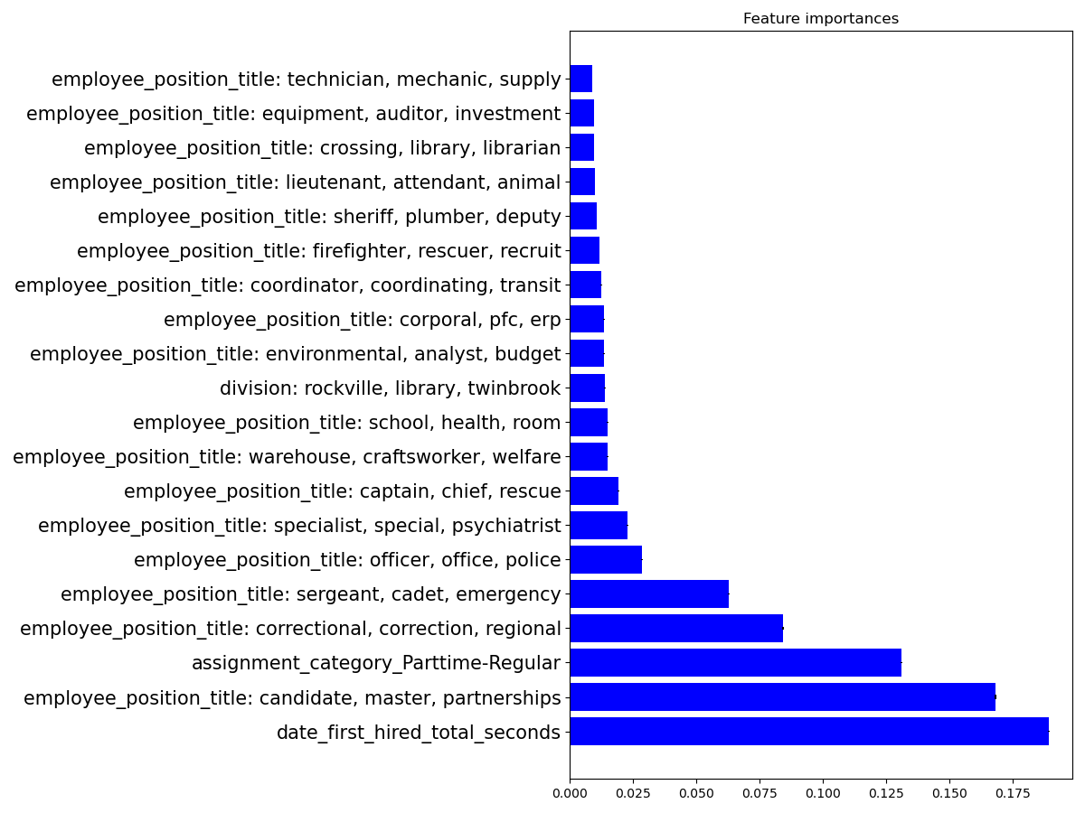
The GapEncoder creates feature names that show the first 3 most important words in
the topic associated with each feature. As we can see in the plot above, this helps
inspecting the model. If we had used a MinHashEncoder instead, the features would be
much less helpful, with names such as employee_position_title_0,
employee_position_title_1, etc.
We can see that features such the time elapsed since being hired, having a full-time
employment, and the position, seem to be the most informative for prediction. However,
feature importances must not be over-interpreted – they capture statistical
associations rather than causal effects. Moreover, the
fast feature importance method used here suffers from biases favouring features with
larger cardinality, as illustrated in a scikit-learn example.
In general we should prefer permutation_importance(), but it is a slower method.
Conclusion#
In this example, we motivated the need for a simple machine learning
pipeline, which we built using the TableVectorizer and a
HistGradientBoostingRegressor.
We saw that by default, it works well on a heterogeneous dataset.
To better understand our dataset, and without much effort, we were also able to plot the feature importances.
Total running time of the script: (0 minutes 49.450 seconds)