Feature interpretation with the GapEncoder

In this notebook, we will explore the output and inner workings of the GapEncoder, one of the high cardinality categorical encoders provided by skrub.

The GapEncoder is scalable and interpretable in terms of finding latent categories, as we will show.

First, let’s retrieve the employee salaries dataset:

from skrub.datasets import fetch_employee_salaries

dataset = fetch_employee_salaries()

# Alias X and y
X, y = dataset.X, dataset.y

X

	gender	department	department_name	division	assignment_category	employee_position_title	date_first_hired	year_first_hired
0	F	POL	Department of Police	MSB Information Mgmt and Tech Division Records...	Fulltime-Regular	Office Services Coordinator	09/22/1986	1986
1	M	POL	Department of Police	ISB Major Crimes Division Fugitive Section	Fulltime-Regular	Master Police Officer	09/12/1988	1988
2	F	HHS	Department of Health and Human Services	Adult Protective and Case Management Services	Fulltime-Regular	Social Worker IV	11/19/1989	1989
3	M	COR	Correction and Rehabilitation	PRRS Facility and Security	Fulltime-Regular	Resident Supervisor II	05/05/2014	2014
4	M	HCA	Department of Housing and Community Affairs	Affordable Housing Programs	Fulltime-Regular	Planning Specialist III	03/05/2007	2007
...	...	...	...	...	...	...	...	...
9223	F	HHS	Department of Health and Human Services	School Based Health Centers	Fulltime-Regular	Community Health Nurse II	11/03/2015	2015
9224	F	FRS	Fire and Rescue Services	Human Resources Division	Fulltime-Regular	Fire/Rescue Division Chief	11/28/1988	1988
9225	M	HHS	Department of Health and Human Services	Child and Adolescent Mental Health Clinic Serv...	Parttime-Regular	Medical Doctor IV - Psychiatrist	04/30/2001	2001
9226	M	CCL	County Council	Council Central Staff	Fulltime-Regular	Manager II	09/05/2006	2006
9227	M	DLC	Department of Liquor Control	Licensure, Regulation and Education	Fulltime-Regular	Alcohol/Tobacco Enforcement Specialist II	01/30/2012	2012

9228 rows × 8 columns

Encoding job titles

Let’s look at the job titles, the column containing dirty data we want to encode:

Note:

Dirty data, as opposed to clean, are all non-curated categorical columns with variations such as typos, abbreviations, duplications, alternate naming conventions etc.

X_dirty = X["employee_position_title"]

Let’s have a look at a sample of the job titles:

X_dirty.sort_values().tail(15)

7753     Work Force Leader II
1231     Work Force Leader II
3206     Work Force Leader II
2602     Work Force Leader II
6872    Work Force Leader III
3601    Work Force Leader III
6922     Work Force Leader IV
502      Work Force Leader IV
3469     Work Force Leader IV
353      Work Force Leader IV
5838     Work Force Leader IV
4961     Work Force Leader IV
2766     Work Force Leader IV
4556     Work Force Leader IV
7478     Work Force Leader IV
Name: employee_position_title, dtype: object

Then, we create an instance of the GapEncoder with 10 components. This means that the encoder will attempt to extract 10 latent topics from the input data:

from skrub import GapEncoder

enc = GapEncoder(n_components=10, random_state=1)

Finally, we fit the model on the dirty categorical data and transform it in order to obtain encoded vectors of size 10:

X_enc = enc.fit_transform(X_dirty)
X_enc.shape

(9228, 10)

Interpreting encoded vectors

The GapEncoder can be understood as a continuous encoding on a set of latent topics estimated from the data. The latent topics are built by capturing combinations of substrings that frequently co-occur, and encoded vectors correspond to their activations. To interpret these latent topics, we select for each of them a few labels from the input data with the highest activations. In the example below we select 3 labels to summarize each topic.

topic_labels = enc.get_feature_names_out(n_labels=3)
for k, labels in enumerate(topic_labels):
    print(f"Topic n°{k}: {labels}")

Topic n°0: employee_position_title: administrative, administration, legislative
Topic n°1: employee_position_title: equipment, operator, liquor
Topic n°2: employee_position_title: correctional, correction, officer
Topic n°3: employee_position_title: firefighter, rescuer, rescue
Topic n°4: employee_position_title: technology, technician, mechanic
Topic n°5: employee_position_title: enforcement, crossing, warehouse
Topic n°6: employee_position_title: manager, worker, program
Topic n°7: employee_position_title: communications, community, safety
Topic n°8: employee_position_title: specialist, special, planning
Topic n°9: employee_position_title: services, supervisor, coordinator

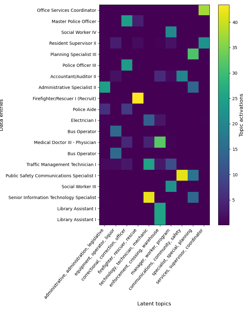
As expected, topics capture labels that frequently co-occur. For instance, the labels “firefighter”, “rescuer”, “rescue” appear together in “Firefighter/Rescuer III”, or “Fire/Rescue Lieutenant”.

We can now understand the encoding of different samples.

import matplotlib.pyplot as plt

encoded_labels = enc.transform(X_dirty[:20])
plt.figure(figsize=(8, 10))
plt.imshow(encoded_labels)
plt.xlabel("Latent topics", size=12)
plt.xticks(range(0, 10), labels=topic_labels, rotation=50, ha="right")
plt.ylabel("Data entries", size=12)
plt.yticks(range(0, 20), labels=X_dirty[:20].to_numpy().flatten())
plt.colorbar().set_label(label="Topic activations", size=12)
plt.tight_layout()
plt.show()

As we can see, each dirty category encodes on a small number of topics, These can thus be reliably used to summarize each topic, which are in effect latent categories captured from the data.

Conclusion

In this notebook, we have seen how to interpret the output of the GapEncoder, and how it can be used to summarize categorical variables as a set of latent topics.