Spatial join for flight data: Joining across multiple columns#

Joining tables may be difficult if one entry on one side does not have an exact match on the other side.

This problem becomes even more complex when multiple columns are significant for the join. For instance, this is the case for spatial joins on two columns, typically longitude and latitude.

Joiner() is a scikit-learn compatible transformer that enables performing joins across multiple keys, independantly of the data type (numerical, string or mixed).

The following example uses US domestic flights data to illustrate how space and time information from a pool of tables are combined for machine learning.

Flight-delays data#

The goal is to predict flight delays. We have a pool of tables that we will use to improve our prediction.

The following tables are at our disposal:

The main table: flights dataset#

  • The flights datasets. It contains all US flights date, origin and destination airports and flight time. Here, we consider only flights from 2008.

import pandas as pd
from skrub.datasets import fetch_figshare

flights = fetch_figshare("41771418").X
# Sampling for faster computation.
flights = flights.sample(20_000, random_state=1, ignore_index=True)
flights.head()
Year_Month_DayofMonth DayOfWeek CRSDepTime CRSArrTime UniqueCarrier FlightNum TailNum CRSElapsedTime ArrDelay Origin Dest Distance
0 2008-01-13 7 1900-01-01 18:35:00 1900-01-01 20:08:00 CO 150 N17244 213.0 1.0 IAH ONT 1334.0
1 2008-02-21 4 1900-01-01 14:30:00 1900-01-01 16:06:00 NW 807 N590NW 216.0 2.0 MSP SEA 1399.0
2 2008-04-17 4 1900-01-01 09:40:00 1900-01-01 13:15:00 WN 1684 N642WN 155.0 -13.0 SEA DEN 1024.0
3 2008-01-03 4 1900-01-01 08:40:00 1900-01-01 12:03:00 CO 287 N21723 383.0 46.0 EWR SNA 2433.0
4 2008-01-31 4 1900-01-01 12:50:00 1900-01-01 14:10:00 MQ 3157 N848AE 80.0 -14.0 SJC SNA 342.0


Let us see the arrival delay of the flights in the dataset:

import matplotlib.pyplot as plt
import seaborn as sns

sns.set_theme(style="ticks")

ax = sns.histplot(data=flights, x="ArrDelay")
ax.set_yscale("log")
plt.show()
07 multiple key join

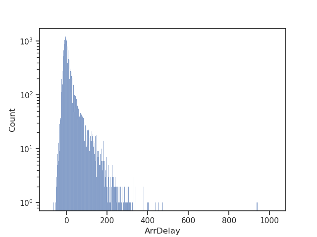
Interesting, most delays are relatively short (<100 min), but there are some very long ones.

Airport data: an auxiliary table from the same database#

  • The airports dataset, with information such as their name and location (longitude, latitude).

airports = fetch_figshare("41710257").X
airports.head()
iata airport city state country lat long
0 00M Thigpen Bay Springs MS USA 31.953765 -89.234505
1 00R Livingston Municipal Livingston TX USA 30.685861 -95.017928
2 00V Meadow Lake Colorado Springs CO USA 38.945749 -104.569893
3 01G Perry-Warsaw Perry NY USA 42.741347 -78.052081
4 01J Hilliard Airpark Hilliard FL USA 30.688012 -81.905944


Weather data: auxiliary tables from external sources#

  • The weather table. Weather details by measurement station. Both tables are from the Global Historical Climatology Network. Here, we consider only weather measurements from 2008.

weather = fetch_figshare("41771457").X
# Sampling for faster computation.
weather = weather.sample(100_000, random_state=1, ignore_index=True)
weather.head()
ID YEAR/MONTH/DAY TMAX PRCP SNOW
0 ASN00041037 2008-06-18 NaN 0.0 NaN
1 USC00164696 2008-01-04 39.0 0.0 0.0
2 US1ILSP0008 2008-08-19 NaN 0.0 0.0
3 USC00164931 2008-10-05 NaN 0.0 0.0
4 NOE00111309 2008-08-18 NaN 0.0 NaN


  • The stations dataset. Provides location of all the weather measurement stations in the US.

stations = fetch_figshare("41710524").X
stations.head()
ID LATITUDE LONGITUDE ELEVATION STATE NAME GSN FLAG HCN/CRN FLAG WMO ID
0 ACW00011604 17.1167 -61.7833 10.1 ST JOHNS COOLIDGE FLD None None NaN NaN
1 ACW00011647 17.1333 -61.7833 19.2 ST JOHNS None None NaN NaN
2 AE000041196 25.3330 55.5170 34.0 SHARJAH INTER. AIRP None GSN 41196.0 NaN
3 AEM00041194 25.2550 55.3640 10.4 DUBAI INTL None None 41194.0 NaN
4 AEM00041217 24.4330 54.6510 26.8 ABU DHABI INTL None None 41217.0 NaN


Joining: feature augmentation across tables#

First we join the stations with weather on the ID (exact join):

ID LATITUDE LONGITUDE ELEVATION STATE NAME GSN FLAG HCN/CRN FLAG WMO ID YEAR/MONTH/DAY TMAX PRCP SNOW
0 AE000041196 25.333 55.517 34.0 SHARJAH INTER. AIRP None GSN 41196.0 NaN 2008-08-15 422.0 0.0 NaN
1 AE000041196 25.333 55.517 34.0 SHARJAH INTER. AIRP None GSN 41196.0 NaN 2008-05-08 374.0 0.0 NaN
2 AEM00041194 25.255 55.364 10.4 DUBAI INTL None None 41194.0 NaN 2008-04-04 288.0 0.0 NaN
3 AEM00041194 25.255 55.364 10.4 DUBAI INTL None None 41194.0 NaN 2008-05-21 365.0 0.0 NaN
4 AEM00041194 25.255 55.364 10.4 DUBAI INTL None None 41194.0 NaN 2008-01-21 221.0 0.0 NaN


Then we join this table with the airports so that we get all auxilliary tables into one.

from skrub import Joiner

joiner = Joiner(airports, aux_key=["lat", "long"], main_key=["LATITUDE", "LONGITUDE"])

aux_augmented = joiner.fit_transform(aux)

aux_augmented.head()
ID LATITUDE LONGITUDE ELEVATION STATE NAME GSN FLAG HCN/CRN FLAG WMO ID YEAR/MONTH/DAY TMAX PRCP SNOW iata airport city state country lat long skrub_Joiner_distance skrub_Joiner_rescaled_distance skrub_Joiner_match_accepted
0 AE000041196 25.333 55.517 34.0 SHARJAH INTER. AIRP None GSN 41196.0 NaN 2008-08-15 422.0 0.0 NaN ROP Prachinburi None None Thailand 14.078333 101.378334 2.418437 3.314381 True
1 AE000041196 25.333 55.517 34.0 SHARJAH INTER. AIRP None GSN 41196.0 NaN 2008-05-08 374.0 0.0 NaN ROP Prachinburi None None Thailand 14.078333 101.378334 2.418437 3.314381 True
2 AEM00041194 25.255 55.364 10.4 DUBAI INTL None None 41194.0 NaN 2008-04-04 288.0 0.0 NaN ROP Prachinburi None None Thailand 14.078333 101.378334 2.418780 3.314851 True
3 AEM00041194 25.255 55.364 10.4 DUBAI INTL None None 41194.0 NaN 2008-05-21 365.0 0.0 NaN ROP Prachinburi None None Thailand 14.078333 101.378334 2.418780 3.314851 True
4 AEM00041194 25.255 55.364 10.4 DUBAI INTL None None 41194.0 NaN 2008-01-21 221.0 0.0 NaN ROP Prachinburi None None Thailand 14.078333 101.378334 2.418780 3.314851 True


Joining airports with flights data: Let’s instanciate another multiple key joiner on the date and the airport:

joiner = Joiner(
    aux_augmented,
    aux_key=["YEAR/MONTH/DAY", "iata"],
    main_key=["Year_Month_DayofMonth", "Origin"],
)

flights.drop(columns=["TailNum", "FlightNum"])
Year_Month_DayofMonth DayOfWeek CRSDepTime CRSArrTime UniqueCarrier CRSElapsedTime ArrDelay Origin Dest Distance
0 2008-01-13 7 1900-01-01 18:35:00 1900-01-01 20:08:00 CO 213.0 1.0 IAH ONT 1334.0
1 2008-02-21 4 1900-01-01 14:30:00 1900-01-01 16:06:00 NW 216.0 2.0 MSP SEA 1399.0
2 2008-04-17 4 1900-01-01 09:40:00 1900-01-01 13:15:00 WN 155.0 -13.0 SEA DEN 1024.0
3 2008-01-03 4 1900-01-01 08:40:00 1900-01-01 12:03:00 CO 383.0 46.0 EWR SNA 2433.0
4 2008-01-31 4 1900-01-01 12:50:00 1900-01-01 14:10:00 MQ 80.0 -14.0 SJC SNA 342.0
... ... ... ... ... ... ... ... ... ... ...
19995 2008-01-14 1 1900-01-01 09:50:00 1900-01-01 11:45:00 WN 115.0 -7.0 SMF SEA 605.0
19996 2008-03-19 3 1900-01-01 13:55:00 1900-01-01 18:40:00 AA 165.0 -27.0 LAS DFW 1055.0
19997 2008-03-15 6 1900-01-01 12:00:00 1900-01-01 18:50:00 WN 230.0 -29.0 PHX PIT 1813.0
19998 2008-02-27 3 1900-01-01 07:20:00 1900-01-01 09:00:00 MQ 100.0 NaN XNA ORD 522.0
19999 2008-03-04 2 1900-01-01 06:20:00 1900-01-01 08:01:00 9E 101.0 -8.0 IAH MEM 469.0

20000 rows × 10 columns


Training data is then passed through a Pipeline:

  • We will combine all the information from our pool of tables into “flights”,

our main table. - We will use this main table to model the prediction of flight delay.

from skrub import TableVectorizer
from sklearn.ensemble import HistGradientBoostingClassifier
from sklearn.pipeline import make_pipeline

tv = TableVectorizer()
hgb = HistGradientBoostingClassifier()

pipeline_hgb = make_pipeline(joiner, tv, hgb)

We isolate our target variable and remove useless ID variables:

y = flights["ArrDelay"]
X = flights.drop(columns=["ArrDelay"])

We want to frame this as a classification problem: suppose that your company is obliged to reimburse the ticket price if the flight is delayed.

We have a binary classification problem: the flight was delayed (1) or not (0).

y = (y > 0).astype(int)
y.value_counts()
ArrDelay
0    10686
1     9314
Name: count, dtype: int64

The results:

from sklearn.model_selection import cross_val_score

scores = cross_val_score(pipeline_hgb, X, y)
scores.mean()
/home/circleci/project/miniconda/envs/testenv/lib/python3.10/site-packages/sklearn/preprocessing/_encoders.py:228: UserWarning: Found unknown categories in columns [1] during transform. These unknown categories will be encoded as all zeros
  warnings.warn(
/home/circleci/project/miniconda/envs/testenv/lib/python3.10/site-packages/sklearn/preprocessing/_encoders.py:228: UserWarning: Found unknown categories in columns [1] during transform. These unknown categories will be encoded as all zeros
  warnings.warn(
/home/circleci/project/miniconda/envs/testenv/lib/python3.10/site-packages/sklearn/preprocessing/_encoders.py:228: UserWarning: Found unknown categories in columns [1] during transform. These unknown categories will be encoded as all zeros
  warnings.warn(

0.58445

Conclusion#

In this example, we have combined multiple tables with complex joins on imprecise and multiple-key correspondences. This is made easy by skrub’s Joiner() transformer.

Our final cross-validated accuracy score is 0.58.

Total running time of the script: (13 minutes 12.928 seconds)

Gallery generated by Sphinx-Gallery